Extending the Cyclostationarity Paradigm from Regular to Irregular Cyclicity

W.A. Gardner

On this page, the reader is provided with a broad perspective on the long history of the modeling of cycles in time series data. Following a unique historical contribution, written by Herman O. A. Wold, in 1968, two further sections are included on advances made following the phase that began in the mid-1980s, when the first comprehensive theory of cyclostationarity was introduced. This entire website is focused on the cyclostationarity phase of research on regular cyclicity that began in the mid-1980s and continues as of today. Pages 4.2 and 4.3, in contrast, provide an introduction to the most recent phase that began in 2015, for which the focus is on irregular cyclicity. This phase was first conceived of by the WCM, but the seminal work was done in partial collaboration between the WCM and Professor Antonio Napolitano, which led to both joint and independent contributions by each of these originators. Page 4.2 presents a published article by the WCM, and Page 4.3 is based on a published article by both originators, and it references a published independent article by Napolitano.

4.1 Evolution of modeling of cycles in Time-series Data
Here is a coarse timeline of the progression of recorded thought about cycles and corresponding data models from basic interest in cycles to the most sophisticated mathematical models yet to be devised:
- 2000 BC: Interest in the General Notion of Cycles [see Wold’s remarks below]
- 1700s AD: Hidden periodicities [Euler, Lagrange; page 2 of [Bk2]]
- 1927: Disturbed Harmonics [Yule; page 14 of [Bk2]]
- 1985 – 1987: Regular Cyclostationarity [first in-depth treatises: Gardner; Chapter 13 of [Bk3] and Part II of [Bk2]]
- 2015 – 2018: Irregular Cyclostationarity [origin: Gardner, [JP65], and Napolitano, [J39]]
The treatment of time-series in [Bk2] is the first to argue that Cyclostationarity modeling is missing from two centuries of work with hidden periodicities and half a century with disturbed harmonics and that, from the mid-20^th Century on, there is no apparent reason for this shortcoming of the time-series analysis body of knowledge other than the convenience of the availability of a mathematical theory of stationary stochastic Stochastic | adjective Involving random variables, as in stochastic process which is a time-indexed sequence of random variables. processes and the fact that a seemingly harmless technique promoted by Blackman and Tukey in 1958 [page 357 of [Bk2]] can be used to render stationary a stochastic process otherwise exhibiting what later became known as cyclostationarity—a property that had been intentionally avoided following the introduction three decades earlier of stochastic processes. This “harmless” technique can indeed be quite harmful in terms of yielding higher-than-minimum-risk statistical Statistical | adjective Of or having to do with Statistics, which are summary descriptions computed from finite sets of empirical data; not necessarily related to probability. inferences based on the time series and its stationary model ([Bk1], [Bk2]), and in terms of masking key properties, such as spectral correlation, and powerful insight into statistical inference involving cycles ([JP19]). In the 1968 article below by H.O.A. Wold, it is acknowledged that interest in the study of cyclicity waned following the transition from classical time-series analysis to the stationary stochastic process framework.

Almost thirty years after writing the first treatise on Regular Cyclostationarity, while the WCM was in formal retirement (dabbling in Electric Universe Theory), he had enough slack in his responsibilities to go back and consider the alternative class of cyclostationarity complementary to regular cyclostationarity: namely irregular cyclostationarity. In 2015, the original unpublished version of the 2018 publication [JP65] revealed how to extend the cyclostationarity paradigm from regular to irregular cyclostationary times series, which are the predominant time series in science where data arises primarily from natural phenomena, not manmade phenomena as is more typically the case in engineering.

Before moving on to this latest development in the study of cyclicity in time-series data–the theory and method for Irregular Cyclicity–historically minded readers may wish to peruse a perspective on pre-cyclostationarity thinking about the modeling of cycles. Such is presented in the form of an excerpt from the International Encyclopedia. This highly readable survey lends insight into the challenge presented to time-series analysts by irregular cyclicity. Consequently, it is to be expected that it will take a fair amount of time with experimentation for the value of this latest development in methodology, presented in [JP65] and summarized in Section 4.2, to emerge.

Note from WCM: The worldwide web source of this article, which is all I had access to at the time of this posting, does not include the figures and equations from the original article. For this reason, the last three sections (relatively short in length) are omitted here because they are mostly unintelligible without the equations. However, the bulk of the article which is included reads very well without the figures. The omitted sections are: Mathematical analysis (“The verbal exposition will now, in all brevity, be linked up with the theory of stochastic processes”); Generalizations. (“The scheme (3) extends to several hidden periodicities”); Stationary stochastic processes. (“The above models are fundamental cases of stationary stochastic processes”). In the material included here, there are also apparently a few missing words or mathematical expression—but their absence does not appear to detract from comprehension.

Cycles

by Herman O. A. Wold

International Encyclopedia of the Social Sciences, 1968, Vol 16, pp. 70 – 80, New York: Macmillan

Cycles, waves, pulsations, rhythmic phenomena, regularity in return, periodicity—these notions reflect a broad category of natural, human, and social phenomena where cycles are the dominating feature. The daily and yearly cycles in sunlight, temperature, and other geophysical phenomena are among the simplest and most obvious instances. Regular periodicity provides a basis for prediction and for extracting other useful information about the observed phenomena. Nautical almanacs with their tidal forecasts are a typical example. Medical examples are pulse rate as an indicator of cardiovascular status and the electrocardiograph as a basis for analysis of the condition of the heart.

The study of cyclic phenomena dates from prehistoric times, and so does the experience that the area has dangerous pitfalls. From the dawn of Chinese history comes the story that the astronomers Hi and Ho lost their heads because they failed to forecast a solar eclipse (perhaps 2137 b.c.). In 1929, after some twelve years of promising existence, the Harvard Business Barometer (or Business Index) disappeared because it failed to predict the precipitous drop in the New York stock market.

Cyclic phenomena are recorded in terms of time series. A key aspect of cycles is the degree of predictability they give to the time series generated. Three basic situations should be distinguished:

(a) The cycles are fixed, so that the series is predictable over the indefinite future.

(b) The cycles are partly random, so that the series is predictable only over a limited future.

(c) The cycles are spurious—that is, there are no real cycles—and the series is not predictable.

For the purposes of this article the term “cycle” is used in a somewhat broader sense than the strict cyclic periodicity of case (a).

Limited and unlimited predictability

The fundamental difference between situations (a) and (b) can be illustrated by two simple cases.

The scheme of “hidden periodicities.” Suppose that an observed time series is generated by two components. The first is strictly periodic, with period length p, so that its value at time t + p is equal to its value at time t. The second component, superimposed upon the first, is a sequence of random (independent, identically distributed) elements. Thus, each term of the observed series can be represented as the sum of a periodic term and a random one.

Tidal water is a cyclic phenomenon where this model applies quite well (see Figure 1). Here the observed series is the measured water level at Dover, the strictly periodic component represents the lunar cycle, 12 hours and 50 minutes in length (two maxima in one lunar day), and the random elements are the irregular deviations caused by storms, random variations in air pressure, earthquakes, etc.

The periodic component provides a prediction—

Hypothetical data. An unbiased predicted value for a future time with expectation equal to that future value of the periodic component, and with prediction error equal to the random Random | adjectiveUnpredictable, but not necessarily modeled in terms of probability and not necessarily stochastic. element. The difficulty is that the periodic component is not known and must be estimated empirically. A simple and obvious method is that of Buys Ballot’s table; each point on the periodic component is estimated by the average of several points on the observed series, separated in time by the length of the period, p, where p either is known or is assessed by trial and error. The larger is the residual as compared to the cyclic component, the longer is the series needed to estimate with confidence the cyclic component.

The approach of hidden periodicities may be extended, with two or more periodic components being considered. Tidal water again provides a typical illustration. In addition to the dominating lunar component, a closer fit to the data is obtained by considering a solar component with period 183 days.

In view of its simplicity and its many important applications, it is only natural that the approach involving strictly periodic components is of long standing. A distinction must be made, however, between formal representation of a series (which is always possible), on the one hand, and prediction, on the other. Under general conditions, any series, even a completely random one, can be represented by a sum of periodic components plus a residual, and if the number of periodic components is increased indefinitely, the residual can be made as small as desired. In particular, if each of the periodic components is a sine or a cosine curve (a sinusoid), then the representation of the observed series is called a spectral representation. Such a representation, it is well to note, may be of only limited use for prediction outside the observed range, because if the observed range is widened, the terms of the representation may change appreciably. In the extreme case when the observations are all stochastically independent, the spectral representation of the series is an infinite sum of sinusoids; in this case neither the spectral representation nor alternative forecasting devices provide any predictive information.

Irregular cycles. Until rather recently (about 1930), the analysis of oscillatory time series was almost equivalent to the assessment of periodicities. For a long time, however, it had been clear that important phenomena existed that refused to adhere to the forecasts based on the scheme of hidden periodicities. The most obvious and challenging of these was the sequence of some twenty business cycles, each of duration five to ten years, between 1800 and 1914. Phenomena with irregular cycles require radically different methods of analysis.

The scheme of “disturbed periodicity.” The breakthrough in the area of limited predictability came with Yule’s model (1927) for the irregular 11-year cycle of sunspot intensity (see Figure 2). Yule interpreted the sunspot cycle as similar to the movement of a damped pendulum that is kept in motion by an unending stream of random shocks. [See the biography of Yule.]

The sharp contrast between the scheme of hidden periodicities and the scheme of disturbed periodicity can now be seen. In the hidden periodicities model the random elements are superimposed upon the cyclic component(s) without affecting or disturbing their strict periodicity. In Yule’s model the series may be regarded as generated by the random elements, and there is no room for strict periodicity. (Of course, the two types can be combined, as will be seen.)

The deep difference between the two types of model is reflected in their forecasting properties (see Figure 3). The time scales for the two forecasts have here been adjusted so as to give the same period. In the hidden-periodicities model the forecast over the future time span has the form of an undamped sinusoid, thus permitting an effective forecast over indefinitely long spans when the model is correct. In Yule’s model the forecast is a damped sinusoid, which provides effective information over limited spans, but beyond that it gives only the trivial forecast that the value of the series is expected to equal the unconditional over-all mean of the series.

Generalizations. The distinction between limited and unlimited predictability of an observed times series goes to the core of the probability structure of the series.

In the modern development of time series analysis on the basis of the theory of stochastic processes, the notions of predictability are brought to full significance. It can be shown that the series y_t under very general conditions allows a unique representation,

known as predictive decomposition, where (a) the two components are uncorrelated, (b) Φ_t is deterministic and Ψ_t is nondeterministic, and (c) the nondeterministic component allows a representation of the Yule type. In Yule’s model no Φ_t component is present. In the hidden-periodicities model Φ_t, is a sum of sinusoids, while Ψ_t is the random Φ_t residual. Generally, however, Φ_t although deterministic in the prediction sense, is random.

The statistical treatment of mixed models like (1) involves a variety of important and challenging problems. Speaking broadly, the valid assessment of the structure requires observations that extend over a substantial number of cycles, and even then the task is difficult. A basic problem is to test for and estimate a periodic component on the supplementary hypothesis that the ensuing residual allows a nondeterministic representation, or, more generally, to perform a simultaneous estimation of the two components. A general method for dealing with these problems has been provided by Whittle (1954); for a related approach, see Allais (1962).

Other problems with a background in this decomposition occur in the analysis of seasonal variation [See Time series, article on Seasonal adjustment].

Other stochastic models. Since a tendency to cyclic variation is a conspicuous feature of many phenomena, stochastic models for their analysis have used a variety of mechanisms for generating apparent or genuine cyclicity. Brief reference will be made to the dynamic models for (a) predator-prey populations and (b) epidemic diseases. In both cases the pioneering approaches were deterministic, the models having the form of differential equation systems. The stochastic models developed at a later stage are more general, and they cover features of irregularity that cannot be explained by deterministic methods. What is of special interest in the present context is that the cycles produced in the simplest deterministic models are strictly periodic, whereas the stochastic models produce irregular cycles that allow prediction only over a limited future.

Figure 4 refers to a stochastic model given by M. S. Bartlett (1957) for the dynamic balance between the populations of a predator—for example, the lynx—and its prey—for example, the hare. The data of the graph are artificial, being constructed from the model by a Monte Carlo experiment. The classic models of A. J. Lotka and V. Volterra are deterministic, and the ensuing cycles take the form

of sinusoids. The cyclic tendency is quite pronounced in Figure 4, but at the same time the development is affected by random features. After three peaks in both populations, the prey remains at a rather low level that turns out to be critical for the predator, and the predator population dies out.

The peaks in Figure 5 mark the severe spells of poliomyelitis in Sweden from 1905 onward. The cyclic tendency is explained, on the one hand, by the contagious nature of the disease and, on the other, by the fact that slight infections provide immunity, so that after a nationwide epidemic it takes some time before a new group of susceptibles emerges. The foundations for a mathematical theory of the dynamics of epidemic diseases were laid by Kermack and McKendrick (1927), who used a deterministic approach in terms of differential equations. Their famous threshold theorem states that only if the infection rate, ρ, is above a certain critical value, ρ_o, will the disease flare up in epidemics. Bartlett (1957) and others have developed the theory in terms of stochastic models; a stochastic counterpart to the threshold theorem has been provided by Whittle (1955).

Bartlett’s predator-prey model provides an example of how a cyclic deterministic model may become evolutive (nonstationary) when stochasticized, while Whittle’s epidemic model shows how an evolutive deterministic model may become stationary. Both of the stochastic models are completely nondeterministic; note that the predictive decomposition (1) extends to nonstationary processes.

The above examples have been selected so as to emphasize that there is no sharp demarcation between cycles with limited predictability and the spurious periodicity of phenomena ruled by randomness, where by pure chance the variation may take wavelike forms, but which provides no basis even for limited predictions. Thus, if a recurrent phenomenon has a low rate of incidence, say λ per year, and the incidences are mutually independent (perhaps a rare epidemic disease that has no aftereffect of immunity), the record of observations might evoke the idea that the recurrences have some degree of periodicity. It is true that in such cases there is an average period of length 1/λ between the recurrences, but the distance from one recurrence to the next is a random variable that cannot be forecast, since it is independent of past observations.

A related situation occurs in the summation of mutually independent variables. Figure 6 shows a case in point as observed in a Monte Carlo experiment with summation of independent variables (Wold 1965). The similarity between the three waves, each representing the consecutive additions

of some 100,000 variables, is rather striking. Is it really due to pure chance? Or is the computer simulation of the “randomness” marred by some slip that has opened the door to a cyclic tendency in the ensuing sums? (For an amusing discussion of related cases, see Cole’s “Biological Clock in the Unicorn” 1957.)

Figure 6 also gives, in the series of wholesale prices in Great Britain, an example of “Kondratieff waves”—the much discussed interpretation of economic phenomena as moving slowly up and down in spells of some fifty years. Do the waves embody genuine tendencies to long cycles, or are they of a spurious nature? The question is easy to pose but difficult or impossible to answer on the basis of available data. The argument that the “Kondratieff waves” are to a large extent parallel in the main industrialized countries carries little weight, in view of international economic connections. The two graphs have been combined in Figure 6 in order to emphasize that with regard to waves of long duration it is always difficult to sift the wheat of genuine cycles from the chaff of spurious periodicity. [See the biography of Kondratieff.]

Genuine versus spurious cycles

Hypothesis testing. Cycles are a specific feature in many scientific models, and their statistical assessment usually includes (a) parameter estimation for purposes of quantitative specification of the model, and (b) hypothesis testing for purposes of establishing the validity of the model and thereby of the cycles. In modern statistics it is often (sometimes tacitly) specified that any method under (a) should be supplemented by an appropriate device under (b). Now, this principle is easy to state, but it is sometimes difficult to fulfill, particularly with regard to cycles and related problems of time series analysis. The argument behind this view may be summed up as follows, although not everyone would take the same position:

(i) Most of the available methods for hypothesis testing are designed for use in controlled experiments—the supreme tool of scientific model building—whereas the assessment of cycles typically refers to nonexperimental situations.

(ii)The standard methods for both estimation and hypothesis testing are based on the assumption of independent replications. Independence is on the whole a realistic and appropriate assumption in experimental situations, but usually not for non-experimental data.

(iii)Problems of point estimation often require less stringent assumptions than those of interval estimation and hypothesis testing. This is frequently overlooked by the methods designed for experimental applications, because the assumption of independence is usually introduced jointly for point estimation, where it is not always needed, and for hypothesis testing, where it is always consequential.

(iv)It is therefore a frequent situation in the analysis of nonexperimental data that adequate methods are available for estimation, but further assumptions must be introduced to conduct tests of hypotheses. It is even a question whether such tests can be performed at all in a manner corresponding to the standard methods in experimental analysis, because of the danger of specification errors that mar the analysis of nonexperimental data.

(v)Standard methods of hypothesis testing in controlled experiments are thus of limited scope in nonexperimental situations. Here other approaches come to the fore. It will be sufficient to mention predictive testing—the model at issue is taken as a basis for forecasts, and in due course the forecasts are compared with the actual developments. Reporting of nonexperimental models should always include a predictive test.

The following example is on the cranky side, but it does illustrate that the builder of a nonexperimental model should have le courage de son modele to report a predictive test, albeit in this case the quality of the model does not come up to the model builder’s courage. The paper (Lewin 1958) refers to two remarkable events—the first permanent American settlement at Jamestown, Virginia, in 1607 and the Declaration of Independence in 1776 —and takes the 169 years in between as the basic “cycle.” After another 84½% years (½ of the basic cycle) there is the remarkable event of the Civil War, in 1861; after 56 more years (⅓ of the cycle) there is the beginning of the era of world wars in 1917; after 28 more years (1/6 of the cycle) there is the atomic era with the first bomb exploded in 1945. The paper, published in 1958, ends with the following predictive statement: “The above relation to the basic 169-year cycle of 1/1, ½, ⅓ 1/6 is a definite decreasing arithmetic progression where the sum of all previous denominators becomes the denominator of the next fraction. To continue this pattern and project, we have the 6th cycle—1959, next U.S. Epochal Event—14-year lapse— 1/12 of 169 years” (Lewin 1958, pp. 11-12). The 1959 event should have been some major catastrophe like an atomic war, if I have correctly understood what the author intimates between the lines in the first part of his article.

It is well to note that this paper, singled out here as an example, is far from unique. Cycles have an intrinsic fascination for the human mind. A cursory scanning of the literature, particularly Cycles, the journal of the Foundation for the Study of Cycles, will suffice to show that in addition to the strictly scientific contributions, there is a colorful subvegetation where in quality and motivation the papers and books display all shades of quasi-scientific and pseudoscientific method, down to number mysticism and other forms of dilettantism and crankiness, and where the search for truth is sometimes superseded by drives of self-realization and self-suggestion, not to speak of unscrupulous money-making. The crucial distinction here is not between professional scientists and amateurs. It is all to the good if the search for truth is strengthened by many modes of motivation. The sole valid criterion is given by the general standards of scientific method. Professionals are not immune to self-suggestion and other human weaknesses, and the devoted work of amateurs guided by an uncompromising search for truth is as valuable here as in any other scientific area.

Further remarks

Cycles are of key relevance in the theory and application of time series analysis; their difficulty is clear from the fact that it is only recently that scientific tools appropriate for dealing with cycles and their problems have been developed. The fundamental distinction between the hidden-periodicity model, with its strict periodicity and unlimited predictability, and Yule’s model, with its disturbed periodicity and limited predictability, could be brought to full significance only after 1933, by the powerful methods of the modern theory of stochastic processes.

Note from WCM: On the basis of the FOT theory and methodology treated in this website as an alternative to stochastic process theory, the veracity of the above phrase following the words “could be brought to full significance” is questionable—the only randomness in the stochastic models discussed by Wold that cannot be incorporated in this alternative are those which render the stochastic processes non-ergodic; namely, the time-invariant random parameters in the models discussed.

On the applied side, the difficulty of the problems has been revealed in significant shifts in the very way of viewing and posing the problems. Thus, up to the failure of the Harvard Business Barometer the analysis of business cycles was essentially a unirelational approach, the cycle being interpreted as generated by a leading series by way of a system of lagged relationships with other series. The pioneering works of Jan Tinbergen in the late 1930s broke away from the unirelational approach. The models of Tinbergen and his followers are multirelational, the business cycles being seen as the resultant of a complex system of economic relationships. [See Business cycles; Distributed lags.]

The term “cycle,” when used without further specification, primarily refers to periodicities in time series, and that is how the term is taken in this article. The notion of “life cycle” as the path from birth to death of living organisms is outside the scope of this presentation. So are the historical theories of Spengler and Toynbee that make a grandiose combination of time series and life cycle concepts, seeing human history as a succession of cultures that are born, flourish, and die. Even the shortest treatment of these broad issues would carry us far beyond the realm of time series analysis; this omission, however, must not be construed as a criticism. [For a discussion of these issues, see Periodization.]

Cycles vs. innovations. The history of human knowledge suggests that belief in cycles has been a stumbling block in the evolution of science. The philosophy of the cosmic cycle was part of Stoic and Epicurean philosophy: every occurrence is a recurrence; history repeats itself in cycles, cosmic cycles; all things, persons, and phenomena return exactly as before in cycle after cycle. What is it in this strange theory that is of such appeal that it should have been incorporated into the foundations of leading philosophical schools and should occur in less extreme forms again and again in philosophical thinking through the centuries, at least up to Herbert Spencer, although it later lost its vogue? Part of the answer seems to be that philosophy has had difficulties with the notion of innovation, having, as it were, a horror innovationum. If our philosophy leaves no room for innovations, we must conclude that every occurrence is a recurrence, and from there it is psychologically a short step to the cosmic cycle. This argument being a blind alley, the way out has led to the notions of innovation and limited predictability and to other key concepts in modern theories of cyclic phenomena. Thus, in Yule’s model (Figure 2) the random shocks are innovations that reduce the regularity of the sunspot cycles so as to make them predictable only over a limited future. More generally, in the predictive decomposition (1) the nondeterministic component is generated by random elements, innovations, and the component is therefore only of limited predictability. Here there is a close affinity to certain aspects of the general theory of knowledge. We note that prediction always has its cognitive basis in regularities observed in the past, cyclic or not, and that innovations set a ceiling to prediction by scientific methods. [See Time series, article on Advanced problems.]

This article aims at a brief orientation to the portrayal of cycles as a broad topic in transition. Up to the 1930s the cyclical aspects of time series were dealt with by a variety of approaches, in which nonscientific and prescientific views were interspersed with the sound methods of some few forerunners and pioneers.

Note from WCM: The following paragraph has been emphasized with bold font by the WCM; it is suggested that readers consider the following: The WCM proposes that the interest in cycles being superseded as time-series analysis transitioned to the stochastic-process framework, as described below by Wold in 1968, is a result of the fact that the stationary process model, with the possible addition of sinewaves, is simply not appropriate for most cyclic phenomena; the supersession is not a result of cyclicity in data no longer being of interest. This is fairly clear from the huge growth in research on cyclicity in data since the advent of the theory and method of cyclostationarity a couple of decades later.

The mathematical foundations of probability theory as laid by Kolmogorov in 1933 gave rise to forceful developments in time series analysis and stochastic processes, bringing the problems about cycles within the reach of rigorous treatment. In the course of the transition, interest in cycles has been superseded by other aspects of time series analysis, notably prediction and hypothesis testing. For that reason, and also because cyclical features appear in time series of very different probability structures, it is only natural that cycles have not (or not as yet) been taken as a subject for a monograph.

Herman Wold

[See also Business cycles and Prediction and forecasting, Economic]

BIBLIOGRAPHY

Allais, Maurice 1962 Test de périodicité: Généralisation du test de Schuster au cas de séries temporelles autocorrelées dans l’hypothése d’un processus de perturbations aleatoires d’un systéme stable. Institut International de Statistique, Bulletin 39, no. 2:143-193.

Bartlett, M. S. 1957 On Theoretical Models for Competitive and Predatory Biological Systems. Biometrika 44:27-42.

Burkhardt, H. 1904 Trigonometrische Interpolation: Mathematische Behandlung periodischer Naturer-scheinungen mit Einschluss ihrer Anwendungen. Volume 2, pages 643-693 in Enzyklopädie der mathe-matischen Wissenschaften. Leipzig: Teubner. → The encyclopedia was also published in French.

Buys Ballot, Christopher H. D. 1847 Les change-mens périodiques de température dépendants de la nature du soleil et de la lune mis en rapport avec le prognostic du temps déduits d’observations Neer-landaises de 1729 á 1846. Utrecht (Netherlands): Kemink.

Cole, Lamont C. 1957 Biological Clock in the Unicorn. Science 125:874-876.

CramÉr, Harald 1940 On the Theory of Stationary Random Processes. Annals of Mathematics2d Series 41:215-230.

Cycles. → Published since 1950 by the Foundation for the Study of Cycles. See especially Volume 15.

Kermack, W. O.; and Mckendrick, A. G. 1927 A Contribution to the Mathematical Theory of Epidemics. Royal Society of London, Proceedings Series A 113: 700-721.

Kermack, W. O.; and Mckendrick, A. G. 1932 Contributions to the Mathematical Theory of Epidemics. Part 2: The Problem of Endemicity. Royal Society of London, Proceedings Series A 138:55-83.

Kermack, W. O.; and Mckendrick, A. G. 1933 Contributions to the Mathematical Theory of Epidemics. Part 3: Further Studies of the Problem of Endemicity. Royal Society of London, Proceedings Series A 141: 94-122.

Keyser, Cassius J. (1922) 1956 The Group Concept. Volume 3, pages 1538-1557 in James R. Newman, The World of Mathematics: A Small Library of the Literature of Mathematics From A’h-Mosé the Scribe to Albert Einstein. New York: Simon & Schuster. → A paperback edition was published in 1962.

Kolmogorov, A. N. (1941) 1953 Sucesiones esta-cionarias en espacios de Hilbert (Stationary Sequences in Hilbert Space). Trabajos de estadistíca 4:55-73, 243-270. → First published in Russian in Volume 2 of the Biulleten Moskovskogo Universiteta.

Lewin, Edward A. 1958 1959 and a Cyclical Theory of History. Cycles 9:11-12.

Mitchell, Wesley C. 1913 Business Cycles. Berkeley: Univ. of California Press. → Part 3 was reprinted by University of California Press in 1959 as Business Cycles and Their Causes.

Piatier, AndrÉ 1961 Statistique et observation eco-nomique. Volume 2. Paris: Presses Universitaires de France.

Schumpeter, Joseph A. 1939 Business Cycles: A Theoretical, Historical, and Statistical Analysis of the Capitalist Process.2 vols. New York and London: McGraw-Hill. → An abridged version was published in 1964.

Schuster, Arthur 1898 On the Investigation of Hidden Periodicities With Application to a Supposed 26 Day Period of Meteorological Phenomena. Terrestrial Magnetism 3:13-41.

Tinbergen, J. 1940 Econometric Business Cycle Research. Review of Economic Studies 7:73-90.

Whittaker, E. T.; and Robinson, G. (1924) 1944 The Calculus of Observations: A Treatise on Numerical Mathematics.4th ed. Princeton, N.J.: Van Nostrand.

Whittle, P. 1954 The Simultaneous Estimation of a Time Series: Harmonic Components and Covariance Structure. Trabajos de estadistíca 3:43-57.

Whittle, P. 1955 The Outcome of a Stochastic Epidemic—A Note on Bailey’s Paper. Biometrika 42: 116-122.

Wiener, Norbert (1942) 1964 Extrapolation, Interpolation and Smoothing of a Stationary Time Series, With Engineering Applications. Cambridge, Mass.: Technology Press of M.I.T. → First published during World War II as a classified report to Section D2, National Defense Research Committee. A paperback edition was published in 1964.

Wold, Herman (1938) 1954 A Study in the Analysis of Stationary Time Series.2d ed. Stockholm: Almqvist & Wiksell.

Wold, Herman 1965 A Graphic Introduction to Stochastic Processes. Pages 7-76 in International Statistical Institute, Bibliography on Time Series and Stochastic Processes. Edited by Herman Wold. Edinburgh: Oliver & Boyd.

Wold, Herman 1967 Time as the Realm of Forecasting. Pages 525-560 in New York Academy of Sciences, Interdisciplinary Perspectives on Time. New York: The Academy.

Yule, G. Udny 1927 On a Method of Investigating Periodicities in Disturbed Series, With Special Reference to Wolfer’s Sunspot Numbers. Royal Society, Philosophical Transactions Series A 226:267-298.
4.2 A Methodology for the Analysis of Irregular Cyclicity
In the paper [JP65], well-known data analysis benefits of cyclostationary signal-processing methodology are extended from regular to irregular statistical Statistical | adjective Of or having to do with Statistics, which are summary descriptions computed from finite sets of empirical data; not necessarily related to probability. cyclicity in scientific data by using statistically inferred time-warping functions. The methodology is nicely summed up in the process-flow diagram below:

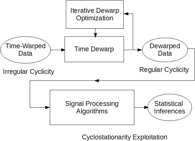
“The devil is in the details”. These details that are at the core of this methodology are contained in the flow box denoted by “Iterative Dewarp Optimization” and are spelled out in [JP65].The following focuses on the introduction to this work.

Abstract

Statistically inferred time-warping functions are proposed for transforming data exhibiting irregular statistical cyclicity (ISC) into data exhibiting regular statistical cyclicity (RSC). This type of transformation enables the application of the theory of cyclostationarity (CS) and polyCS to be extended from data with RSC to data with ISC. The non-extended theory, introduced only a few decades ago, has led to the development of numerous data processing techniques/algorithms for statistical inference that outperform predecessors that are based on the theory of stationarity. So, the proposed extension to ISC data is expected to greatly broaden the already diverse applications of this theory and methodology to measurements/observations of RSC data throughout many fields of engineering and science. This extends the CS paradigm to data with inherent ISC, due to biological and other natural origins of irregular cyclicity. It also extends this paradigm to data with inherent regular cyclicity that has been rendered irregular by time warping due, for example, to sensor motion or other dynamics affecting the data.

The cyclostationarity paradigm in science

Cyclicity is ubiquitous in scientific data: Many dynamical processes encountered in nature arise from periodic or cyclic phenomena. Such processes, although themselves not periodic functions of time, can produce random Random | adjectiveUnpredictable, but not necessarily modeled in terms of probability and not necessarily stochastic. or erratic or otherwise unpredictable data whose statistical characteristics do vary periodically with time and are called cyclostationary (CS) processes. For example, in telecommunications, telemetry, radar, and sonar systems, statistical periodicity or regular cyclicity in data is due to modulation, sampling, scanning, framing, multiplexing, and coding operations. In these information-transmission systems, relative motion between transmitter or reflector and receiver essentially warps the time scale of the received data. Also, if the clock that controls the periodic operation on the data is irregular, the cyclicity of the data is irregular. In mechanical vibration monitoring and diagnosis, cyclicity is due, for example, to various rotating, revolving, or reciprocating parts of rotating machinery; and if the angular speed of motion varies with time, the cyclicity is irregular. However, as explained herein, irregular statistical cyclicity (ISC) due to time-varying RPM or clock timing is not equivalent to time-warped regular statistical cyclicity (RSC). In astrophysics, irregular cyclicity arises from electromagnetically induced revolution and/or rotation of planets, stars, and galaxies and from pulsation and other cyclic phenomena, such as magnetic reversals of planets and stars, and especially Birkeland currents (concentric shells of counter-rotating currents). In econometrics, cyclicity resulting from business cycles has various causes including seasonality and other less regular sources of cyclicity. In atmospheric science, cyclicity is due to rotation and revolution of Earth and other cyclic phenomena affecting Earth, such as solar cycles. In the life sciences, such as biology, cyclicity is exhibited through various biorhythms, such as circadian, tidal, lunar, and gene oscillation rhythms. The study of how solar- and lunar-related rhythms are governed by living pacemakers within organisms constitutes the scientific discipline of chronobiology, which includes comparative anatomy, physiology, genetics, and molecular biology, as well as development, reproduction, ecology, and evolution. Cyclicity also arises in various other fields of study within the physical sciences, such as meteorology, climatology, oceanology, and hydrology. As a matter of fact, the cyclicity in all data is irregular because there are no perfectly regular clocks or pacemakers. But, when the degree of irregularity throughout time-integration intervals required for extracting statistics from data is sufficiently low, the data’s cyclicity can be treated as regular.

The relevance of the theory of cyclostationarity to many fields of time-series analysis was proposed in the mid-1980s in the seminal theoretical work and associated development of data processing methodology reported in [Bk1], [Bk2], [Bk5], which established cyclostationarity as a new paradigm in data modeling and analysis, especially—at that time—in engineering fields and particularly in telecommunications signal processing where the signals typically exhibit RSC. More generally, the majority of the development of such data processing techniques that ensued up to the turn of the century was focused on statistical processing of data with RSC for engineering applications, such as telecommunications/telemetry/radar/sonar and, subsequently, mechanical vibrations of rotating machinery. But today—more than 30 years later—the literature reveals not only expanded engineering applications but also many diverse applications to measurements / observations of RSC data throughout the natural sciences (see Appendix in [JP65]), and it is to be expected there will be many more applications found in the natural sciences for which benefit will be derived from transforming ISC into RSC, and applying the now classical theory and methodology.

The purpose of the paper [JP65] is to enable an extension of the cyclostationarity paradigm from data exhibiting RSC to data exhibiting ISC. The approach taken, when performed in discrete time (as required when implemented digitally), can be classified as adaptive non-uniform resampling of data, and the adaptation proposed is performed blindly (requires no training data) using a property-restoral technique specifically designed to exploit cyclostationarity.

One simple example of a CS signal is described here to illustrate that what is here called regular statistical cyclicity for time-series data can represent extremely erratic behavior relative to a periodic time series. Consider a long train of partially-overlapping pulses or bursts of arbitrary complexity and identical functional form and assume that, for each individual pulse the shape parameters, such as amplitude, width (or time expansion/contraction factor), time-position, and center frequency, are all random variables—their values change unpredictably from one pulse in the train to the next. If these multiple sequences of random parameters associated with the sequence of pulses in the train are jointly stationary random sequences, then the signal is CS and therefore exhibits regular statistical cyclicity, regardless of the fact that the pulse train can be far from anything resembling a periodic signal. As another example, any broadband noise process with center frequency and/or amplitude and/or time scale that is varied periodically is CS. Thus, exactly regular statistical cyclicity can be quite subtle and even unrecognizable to the casual observer. This is reflected in the frequent usage in recent times of CS models for time-series data from natural phenomena of many distinct origins (see Appendix in [JP65]). Yet, there are many ways in which a time-series of even exactly periodic data can be affected by some dynamical process of cycle-time expansion and/or contraction in a manner that renders its statistical cyclicity irregular: not CS or polyCS. The particular type of dynamic process of interest on this page is time warping.

Highlights of Converting Irregular Cyclicity to Regular Cyclicity:
- - Conversion of Irregular Cyclicity in time-series data to Regular Cyclicity is demonstrated
  - Data with Regular Cyclicity can be modeled as Cyclostationary
  - The Cyclostationarity paradigm for statistical inference has proven to be a rich resource
  - Cyclostationarity exploitation offers noise- and interference-tolerant signal processing
  - Cyclostationarity exploitation can now be extended to many more fields of science and engineering
Table of Contents for [JP65]

I. The Cyclostationarity Paradigm in Science
II. Time Warping
III. De-Warping to Restore Cyclostationarity
IV. Warping Compensation Instead of De-Warping
V. Error Analysis
VI. Basis-Function Expansion of De-Warping Function
VII. Inversion of Warping Functions
VIII. Basis-Function Expansion of Warping-Compensation Function
IX. Iterative Gradient-Ascent Search Algorithm
X. Synchronization-Sequence Methods
XI. Pace Irregularity
XII. Design Guidelines
XIII. Numerical Example

The reader is referred to the published article [JP65] for the details of the methodology for the analysis of Irregular Cyclicity. In addition, some stochastic process models for irregular cyclicity are introduced in [J39] and some alternative methods for dewarping are proposed. This latter contribution is discussed in the following section.
4.3 Algorithms for Analysis of Signals with Time-Warped Cyclostationarity

The following article is [J39]:

May 27, 2022

Summary

Two philosophically different approaches to the analysis of signals with imperfect cyclostationarity or imperfect poly-cyclostationarity of the autocorrelation function due to time-warping are compared in [4]. The first approach consists of directly estimating the time-warping function (or its inverse) in a manner that transforms data having an
empirical Empirical Data | noun Numerical quantities derived from observation or measurement in contrast to those derived from theory or logic alone. autocorrelation with irregular cyclicity into data having regular cyclicity [1]. The second approach consists of modeling the signal as a time-warped poly-cyclostationary stochastic Stochastic | adjective Involving random variables, as in stochastic process which is a time-indexed sequence of random variables. process, thereby providing a wide-sense probabilisticProbabilistic | noun Based on the theoretical concept of probability, e.g., a mathematical model of data comprised of probabilities of occurrence of specific data values. characterization–a time-varying probabilistic autocorrelation function–which is used to specify an estimator of the time-warping function that is intended to remove the impact of time-warping [3].

The objective of the methods considered is to restore to time-warped data exhibiting irregular cyclicity the regular cyclicity, called (poly-)cyclostationarity, that data exhibited prior to being time-warped. An important motive for de-warping data is to render the data amenable to signal processing techniques devised specifically for (poly-)cyclostationary signals. But in some applications, the primary motive may be to de-warp data that has been time-warped with an unknown warping function, and the presence of (poly-)cyclostationarity from the data source prior to that data becoming time warped is just happenstance that fortunately provides a means toward the dewarping end.

Time Warping of (Poly-)Cyclostationary Signals

Let $x(t)$ be a wide-sense cyclostationary or poly-cyclostationary signal with periodically (or poly-periodically) time-varying autocorrelation

(1) $\begin{equation*} {\rm E} \left \{ x(t+\tau ) \: x^{(*)}(t) \right \} = \sum _{\alpha \in A} R_{\vetp {x}}^{\alpha }(\tau ) \: e^{j2\pi \alpha t} \: . \end{equation*}$

In (1), $(*)$ denotes optional complex conjugation, subscript $\vet {x} =[x x^{(*)}]$ , and $A$ , depending on $(*)$ , is the countable set of (conjugate) cycle frequencies.

The expectation operator ${\rm E} \{ \cdot \}$ has two interpretations. It is the ensemble average operator in the classical stochastic approach or it is the poly-periodic component extraction operator in the fraction-of-time (FOT) probability approach. In both approaches, which are equivalent in the case of cycloergodicity, the cyclic autocorrelation function $R_{\vetp {x}}^{\alpha }(\tau )$ can be estimated using a finite-time observation by the (conjugate) cyclic correlogram

(2) $\begin{align*} \widehat {R}_{\vetp {x}}^{\alpha }(\tau ) \triangleq \frac {1}{T} \int _{t_0}^{t_0+T} x(t+\tau ) \: x^{(*)}(t) \: e^{-j2\pi \alpha t} \: \mathrm{d} t \: . \end{align*}$

In (2), $x(t)$ is a realization of the stochastic process (with a slight abuse of notation) in the classical stochastic approach or the single function of time in the FOT approach.

Let $\psi (t)$ be an asymptotically unbounded nondecreasing function. The time-warped version of $x(t)$ is given by

(3) $\begin{equation*} y(t) = x(\psi (t)) \: . \end{equation*}$

The time-warped signal $y(t)$ is not poly-CS unless the time warping function $\psi (t)$ is an affine or a poly-periodic function.

In the following sections, two approaches are reviewed to estimate the time warping function or its inverse in order to de-warp $y(t)$ to obtain an estimate of the underlying poly-CS signal. Once this estimate is obtained, cyclostationary signal processing techniques can be used.

Cyclostationarity Restoral

The first approach [1] consists of directly estimating the time-warping function $\psi (t)$ (or its inverse $\psi ^{-1}(t)$ ) in a manner that transforms the data $y(t)$ having an autocorrelation reflecting irregular cyclicity into data having regular cyclicity. Signals are modeled as single functions of time (FOT approach).

Specifically, assuming that $x(t)$ exhibits cyclostationarity with at least one cycle frequency $\alpha _0$ , estimates $\widehat {\psi }$ or $\varphi =\widehat {\psi }^{-1}$ of $\psi$ or $\psi ^{-1}$ are determined such that, for the recovered signal $x_{\varphi }(t)=y(\varphi (t))$ , the amplitude of the complex sine wave at frequency $\alpha _0$ contained in the second-order lag-product $x_{\varphi }(t+\tau ) \: x_{\varphi }^{(*)}(t)$ is maximized.

Let

(4) $\begin{equation*} \left \{ c_k(t) \right \}_{k=1,\dots ,K} \end{equation*}$

be a set of (not necessarily orthonormal) functions. Two procedures are proposed in [1]:

Procedure a) Consider the expansion

(5) $\begin{equation*} \varphi (t) = \widehat {\psi }^{-1}(t) = \mathbf {a}^{\top } \mathbf {c}(t) \end{equation*}$

where $\mathbf {c}(t)=[c_1(t),\dots ,c_{K}(t)]^{\top }$ and $\mathbf {a}=[a_1,\dots ,a_{K}]^{\top }$ , and maximize with respect to $\mathbf {a}$ the objective function

(6) $\begin{equation*} J_{a}(\mathbf {a})=\left | \widehat {R}_{x_{\varphi }}^{\alpha _0}(\tau ) \right |^2 \end{equation*}$

with

(7) $\begin{align*} \widehat {R}_{x_{\varphi }}^{\alpha _0}(\tau ) \triangleq & ~ \frac {1}{T} \int _{t_0}^{t_0+T} \hspace {-6mm} x_{\varphi }(t+\tau ) \: x_{\varphi }^{(*)}(t) \: e^{-j2\pi \alpha _0 t} \: \mathrm{d} t \nonumber \\ = & ~ \frac {1}{T} \int _{t_0}^{t_0+T} \hspace {-6mm} y(\mathbf {a}^{\top }\mathbf {c}(t+\tau )) \: y^{(*)}(\mathbf {a}^{\top }\mathbf {c}(t)) \: e^{-j2\pi \alpha _0 t} \: \mathrm{d} t \qquad \end{align*}$

for some specific value $\alpha _0$ of $\alpha$ . (Generalizations of $J_{a}(\mathbf {a})$ that include sums over $\alpha$ and/or $\tau$ are possible.)

Procedure b) Consider the expansion

(8) $\begin{align*} \widehat {\psi }(t) = & ~ \mathbf {b}^{\top } \mathbf {c}(t) \end{align*}$

where $\mathbf {b}=[b_1,\dots ,b_{K}]^{\top }$ , and maximize with respect to $\mathbf {b}$ the objective function

(9) $\begin{align*} J_{b}(\mathbf {b}) = & ~ \left | \widehat {R}_{x_{\varphi }}^{\alpha _0}(\tau ) \right |^2 \end{align*}$

with

(10) $\begin{align*} \widehat {R}_{x_{\varphi }}^{\alpha _0}(\tau ) = & ~ \frac {1}{T} \int _{\varphi (t_0)}^{\varphi (t_0+T)} \hspace {-6mm} y(u+\Delta _{\varphi }^{\tau }[\varphi ^{-1}(u)]) \: y^{(*)}(u) \: \nonumber \\ & \rule {20mm}{0mm} \cdot e^{-j2\pi \alpha _0 \varphi ^{-1}(u)} \: \TimeDerivative {\dot{\varphi} }^{-1}(u) \: \mathrm{d} u \nonumber \\ \simeq & ~ \frac {1}{T} \int _{t_0}^{t_0+T} \hspace {-6mm} y(u+\tau /\mathbf {b}^{\top }\TimeDerivative {\dot{\mathbf {c}}}(u)) \: y^{(*)}(u) \: \nonumber \\ & \rule {17mm}{0mm} \cdot e^{-j2\pi \alpha _0 \mathbf {b}^{\top }\mathbf {c}(u)} \: \mathbf {b}^{\top }\TimeDerivative {\dot{\mathbf {c}}}(u) \: \mathrm{d} u \end{align*}$

where (10) is obtained from (7) by the variable change $u=\varphi (t)$ and

(11) $\begin{align*} \Delta _{\varphi }^{\tau }[\varphi ^{-1}(u)] \triangleq & ~ \varphi [\varphi ^{-1}(u)+\tau ] -\varphi [\varphi ^{-1}(u)] \nonumber \\ \simeq & ~ \tau [1/\TimeDerivative {\dot{\varphi} }^{-1}(u)] = \tau /\mathbf {b}^{\top }\TimeDerivative {\dot{\mathbf {c}}}(u) \end{align*}$

The value of the vector $\mathbf {a}$ or $\mathbf {b}$ that maximizes the corresponding objective function is taken as an estimate of the coefficient vector for the expansion of $\varphi (t)=\widehat {\psi }^{-1}(t)$ or $\widehat {\psi }(t)$ . The maximization can be performed by a gradient-ascent algorithm, with starting points throughout a sufficiently fine grid.

In both approaches a) and b) data must be re-interpolated in order to evaluate the gradient of the objective function at every iteration of the iterative gradient-ascent search method. This is very time-consuming. However, for $\tau =0$ , method b) does not require data interpolation, and its implementation can be made very efficient. There are several important design parameters, which are discussed in [1].

Characterization and Warping Function Measurements

The second approach [3] consists of modeling the underlying signal $x(t)$ as a time-warped poly-CS stochastic process, thereby providing a wide-sense probabilistic characterization of $y(t)$ in terms of the time-varying autocorrelation function. From this model, an estimator of $\psi (t)$ aimed at removing the impact of time warping is specified. From this estimate, an estimate of the autocorrelation function of the time-warped process is also obtained.

From (1) and (3), the (conjugate) autocorrelation of $y(t)$ immediately follows:

(12) $\begin{align*} {\rm E} \left \{ y(t+\tau ) \: y^{(*)}(t) \right \} = & ~ \sum _{\alpha \in A} R_{\vetp {x}}^{\alpha }\bigl (\psi (t+\tau )-\psi (t)\bigr ) \: e^{j2\pi \alpha \psi (t)} \end{align*}$

A suitable second-order characterization can be obtained by observing that time-warped poly-cyclostationary signals are linear time-variant transformations of poly-cyclostationary signals. Thus, they can be modeled as oscillatory almost-cyclostationary (OACS) signals [2, Sec. 6].

Let us consider the warping function

(13) $\begin{equation*} \psi (t) = t +\epsilon (t) \end{equation*}$

with $\epsilon (t)$ slowly varying, that is,

(14) $\begin{equation*} \sup _{t} \bigl | \: \TimeDerivative {\dot{\epsilon }}(t) \bigr | \ll 1 \: . \end{equation*}$

In such a case, it can be shown that the autocorrelation (12) is closely approximated by

(15) $\begin{equation*} {\rm E} \left \{ y(t+\tau ) \: y^{(*)}(t) \right \} \simeq \sum _{\alpha \in A} e^{j2\pi \alpha \epsilon (t)} \: R_{\vetp {x}}^{\alpha } ( \tau ) \: e^{j2\pi \alpha t} \end{equation*}$

Two methods are proposed in [3] for estimating the function $\epsilon (t)$ .

The first one considers the expansion

(16) $\begin{equation*} \widehat {\epsilon }(t) = \mathbf {e}^{\top } \mathbf {c}(t) \end{equation*}$

where $\mathbf {e}=[e_1,\dots ,e_{K}]^{\top }$ , and provides estimates of the coefficients $e_k$ by maximizing with respect to $\mathbf {e}$ the objective function

(17) $\begin{equation*} J_{e}(\mathbf {e}) \eqdef \int _{\mathcal {T}} \bigl | \widehat {R}_{\mathbf {y}}^{(T)} (\alpha _0,\tau ; \mathbf {e}) \bigr |^2 \: \mathrm{d} \tau \end{equation*}$

where

(18) $\begin{align*} \widehat {R}_{\mathbf {y}}^{(T)} (\alpha _0,\tau ; \mathbf {e}) \triangleq & ~ \frac {1}{T} \int _{t_0-T/2}^{t_0+T/2} y(t+\tau ) \: y^{(*)}(t) \: e^{-j2\pi \alpha _0 t} \: e^{-j2\pi \alpha _0 \mathbf {e}^{\top } \mathbf {c}(t)} \mathrm{d} t \quad \end{align*}$

and $\mathcal {T}$ is a set of values of $\tau$ where $R_{\mathbf {x}}^{\alpha _0}(\tau )$ is significantly non zero. The maximization can be performed by a gradient ascent algorithm. The estimated coefficients are such that the additive-phase factor $e^{j2\pi \alpha _0\epsilon (t)} \: e^{j2\pi \alpha _0 t}$ in the expected lag-product of $y(t)$ (15) is compensated in (17) by using (18).

For the second method, let us define

(19) $\begin{equation*} z^{\alpha _0}(t,\tau ) \triangleq \Bigl [ y(t+\tau ) \: y^{(*)}(t) \: e^{-j2\pi \alpha _0 t} \Bigr ] \otimes h_{W}(t) \end{equation*}$

with $h_{W}(t)$ the impulse-response function of a low-pass filter with monolateral bandwidth $W$ . Under the assumption that the spectral content of the modulated sine waves in (15) do not significantly overlap, and the low-pass filter extracts only one such sine wave, we have that $z^{\alpha _0}(t,\tau ) \simeq R_{\vetp {x}}^{\alpha _0} ( \tau ) \: e^{j2\pi \alpha _0 \epsilon (t)}$ . Therefore, $\epsilon (t)$ can be estimated by

(20) $\begin{equation*} \widehat {\epsilon }(t) = \arg _{\rm uw} \left [ z^{\alpha _0}(t,\tau ) \right ] /(2\pi \alpha _0) \end{equation*}$

to within the unknown constant, where $\arg _{\rm uw}$ denotes the unwrapped phase. This method is also extended in [3] to the case where only a rough estimate of $\alpha _0$ is available.

De-Warping

Once the warping function $\psi (t)$ or its inverse is estimated, the time-warped signal $y(t)$ can be de-warped in order to obtain an estimate $\widehat {x}(t)$ of the underlying poly-cyclostationary signal $x(t)$ . If this dewarping is sufficiently accurate, it renders $\widehat {x}(t)$ amenable to well known signal processing techniques for poly-cyclostationary signals (e.g., FRESH filtering).

If the estimate $\widehat {\psi }^{-1}(t)$ is obtained by the Procedure a) then the estimate of $x(t)$ is immediately obtained as

(21) $\begin{equation*} \widehat {x}(t) = y(\widehat {\psi }^{-1}(t)) \end{equation*}$

which would have already been calculated in (7). In contrast, if the estimate $\widehat {\psi }(t)$ is available by the Procedure b) or by one of the two methods based on the OACS model, the estimate $\widehat {\psi }^{-1}(t)$ should be obtained by inverting $\widehat {\psi }$ .

In the case of $\psi (t) = t +\epsilon (t)$ , with $\epsilon (t)$ slowly varying, it can be shown that a useful estimate of $x(t)$ is [3]

(22) $\begin{equation*} \widehat {x}(t) = y(t-\widehat {\epsilon }(t)) \end{equation*}$

provided that the estimation error is sufficiently small.

References

[1]   W. A. Gardner, “Statistically inferred time warping: extending the cyclostationarity paradigm from regular to irregular statistical Statistical | adjective Of or having to do with Statistics, which are summary descriptions computed from finite sets of empirical data; not necessarily related to probability. cyclicity in scientific data,” EURASIP Journal on Advances in Signal Processing, vol. 2018, no. 1, p. 59, September 2018.
[2]   A. Napolitano, “Cyclostationarity: Limits and generalizations,” Signal Processing, vol. 120, pp. 323–347, March 2016.
[3]   A. Napolitano, “Time-warped almost-cyclostationary signals: Characterization and statistical function measurements,” IEEE Transactions on Signal Processing, vol. 65, no. 20, pp. 5526–5541, October 15 2017.
[4]   A. Napolitano and W. A. Gardner, “Algorithms for analysis of signals with time-warped cyclostationarity,” in 50th Asilomar Conference on Signals, Systems, and Computers, Pacific Grove, California, November 6-9 2016.

4. Extending the Cyclostationarity Paradigm from Regular to Irregular Cyclicity