On this page, the reader is provided with a broad perspective on the long history of the modeling of cycles in time series data. Following a review of the evolution of this field of study on page 4.1, which includes excerpts from a unique historical contribution, written by Herman O. A. Wold, in 1968, sections 4.2 and 4.3 present advances made following the phase that began in the mid-1980s, when the first comprehensive theory of cyclostationarity was introduced. This entire website is focused on the cyclostationarity phase of research on regular cyclicity that began in the mid-1980s and continues as of today. Pages 4.2 and 4.3, in contrast, provide an introduction to the most recent phase that began in 2015, for which the focus is on irregular cyclicity [JP66]. This phase was first conceived by the WCM, but the seminal work was done in partial collaboration between the WCM and Professor Antonio Napolitano, which led to both joint and independent contributions by each of these originators. Page 4.2 presents a published article by the WCM, and Page 4.3 is based on a published article by both originators, and it references a published independent article by Napolitano.
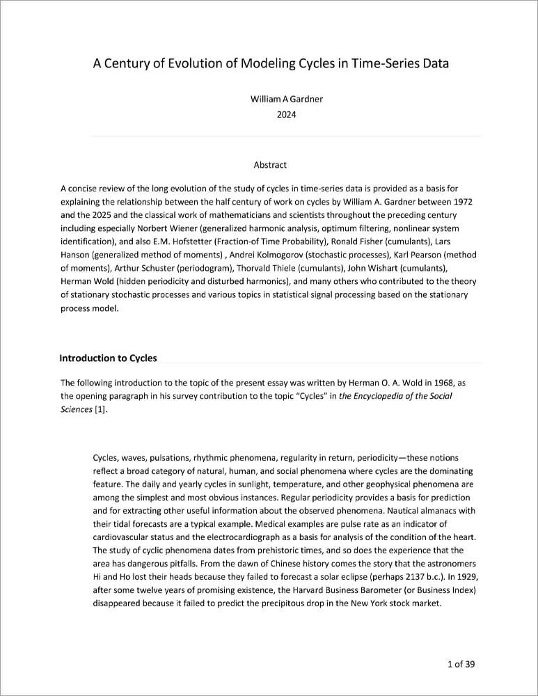
In the essay shown immediately below, a concise review of the long evolution of the study of cycles in time-series data is provided as a basis for explaining the relationship between the half century of work on cycles by the WCM between 1972 and the 2024 and the classical work of mathematicians and scientists throughout the preceding century including especially Norbert Wiener (generalized harmonic analysis, optimum filtering, nonlinear system identification), and also Ronald Fisher (cumulants), Lars Hanson (generalized method of moments), E.M. Hofstetter (Fraction-of-Time Probability), Andrei Kolmogorov (stochastic processes), Karl Pearson (method of moments), Arthur Schuster (periodogram), Thorvald Thiele (cumulants), John Wishart (cumulants), Herman Wold (hidden periodicity and disturbed harmonics), and many others who contributed to the theory of stationary stochastic processes and various topics in statistical signal processing based on the stationary process model.

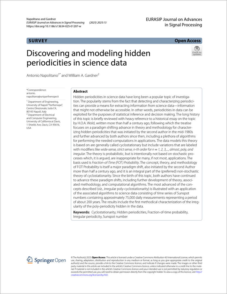
To complement this concise review, a survey paper on hidden periodicity in science data is available here [JP69]:

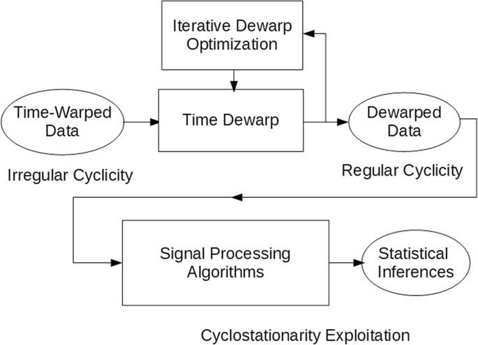
In the paper [JP65], well-known data analysis benefits of cyclostationary signal-processing methodology are extended from regular to irregular statistical Statistical | adjective Of or having to do with Statistics, which are summary descriptions computed from finite sets of empirical data; not necessarily related to probability. cyclicity in scientific data by using statistically inferred time-warping functions. The methodology is nicely summed up in the process-flow diagram below:

“The devil is in the details”. These details that are at the core of this methodology are contained in the flow box denoted by “Iterative Dewarp Optimization” and are spelled out in [JP65].The following focuses on the introduction to this work.
Abstract
Statistically inferred time-warping functions are proposed for transforming data exhibiting irregular statistical cyclicity (ISC) into data exhibiting regular statistical cyclicity (RSC). This type of transformation enables the application of the theory of cyclostationarity (CS) and polyCS to be extended from data with RSC to data with ISC. The non-extended theory, introduced only a few decades ago, has led to the development of numerous data processing techniques/algorithms for statistical inference that outperform predecessors that are based on the theory of stationarity. So, the proposed extension to ISC data is expected to greatly broaden the already diverse applications of this theory and methodology to measurements/observations of RSC data throughout many fields of engineering and science. This extends the CS paradigm to data with inherent ISC, due to biological and other natural origins of irregular cyclicity. It also extends this paradigm to data with inherent regular cyclicity that has been rendered irregular by time warping due, for example, to sensor motion or other dynamics affecting the data.
The cyclostationarity paradigm in science
Cyclicity is ubiquitous in scientific data: Many dynamical processes encountered in nature arise from periodic or cyclic phenomena. Such processes, although themselves not periodic functions of time, can produce random Random | adjectiveUnpredictable, but not necessarily modeled in terms of probability and not necessarily stochastic. or erratic or otherwise unpredictable data whose statistical characteristics do vary periodically with time and are called cyclostationary (CS) processes. For example, in telecommunications, telemetry, radar, and sonar systems, statistical periodicity or regular cyclicity in data is due to modulation, sampling, scanning, framing, multiplexing, and coding operations. In these information-transmission systems, relative motion between transmitter or reflector and receiver essentially warps the time scale of the received data. Also, if the clock that controls the periodic operation on the data is irregular, the cyclicity of the data is irregular. In mechanical vibration monitoring and diagnosis, cyclicity is due, for example, to various rotating, revolving, or reciprocating parts of rotating machinery; and if the angular speed of motion varies with time, the cyclicity is irregular. However, as explained herein, irregular statistical cyclicity (ISC) due to time-varying RPM or clock timing is not equivalent to time-warped regular statistical cyclicity (RSC). In astrophysics, irregular cyclicity arises from electromagnetically induced revolution and/or rotation of planets, stars, and galaxies and from pulsation and other cyclic phenomena, such as magnetic reversals of planets and stars, and especially Birkeland currents (concentric shells of counter-rotating currents). In econometrics, cyclicity resulting from business cycles has various causes including seasonality and other less regular sources of cyclicity. In atmospheric science, cyclicity is due to rotation and revolution of Earth and other cyclic phenomena affecting Earth, such as solar cycles. In the life sciences, such as biology, cyclicity is exhibited through various biorhythms, such as circadian, tidal, lunar, and gene oscillation rhythms. The study of how solar- and lunar-related rhythms are governed by living pacemakers within organisms constitutes the scientific discipline of chronobiology, which includes comparative anatomy, physiology, genetics, and molecular biology, as well as development, reproduction, ecology, and evolution. Cyclicity also arises in various other fields of study within the physical sciences, such as meteorology, climatology, oceanology, and hydrology. As a matter of fact, the cyclicity in all data is irregular because there are no perfectly regular clocks or pacemakers. But, when the degree of irregularity throughout time-integration intervals required for extracting statistics from data is sufficiently low, the data’s cyclicity can be treated as regular.
The relevance of the theory of cyclostationarity to many fields of time-series analysis was proposed in the mid-1980s in the seminal theoretical work and associated development of data processing methodology reported in [Bk1], [Bk2], [Bk5], which established cyclostationarity as a new paradigm in data modeling and analysis, especially—at that time—in engineering fields and particularly in telecommunications signal processing where the signals typically exhibit RSC. More generally, the majority of the development of such data processing techniques that ensued up to the turn of the century was focused on statistical processing of data with RSC for engineering applications, such as telecommunications/telemetry/radar/sonar and, subsequently, mechanical vibrations of rotating machinery. But today—more than 30 years later—the literature reveals not only expanded engineering applications but also many diverse applications to measurements / observations of RSC data throughout the natural sciences (see Appendix in [JP65]), and it is to be expected there will be many more applications found in the natural sciences for which benefit will be derived from transforming ISC into RSC, and applying the now classical theory and methodology.
The purpose of the paper [JP65] is to enable an extension of the cyclostationarity paradigm from data exhibiting RSC to data exhibiting ISC. The approach taken, when performed in discrete time (as required when implemented digitally), can be classified as adaptive non-uniform resampling of data, and the adaptation proposed is performed blindly (requires no training data) using a property-restoral technique specifically designed to exploit cyclostationarity.
One simple example of a CS signal is described here to illustrate that what is here called regular statistical cyclicity for time-series data can represent extremely erratic behavior relative to a periodic time series. Consider a long train of partially-overlapping pulses or bursts of arbitrary complexity and identical functional form and assume that, for each individual pulse the shape parameters, such as amplitude, width (or time expansion/contraction factor), time-position, and center frequency, are all random variables—their values change unpredictably from one pulse in the train to the next. If these multiple sequences of random parameters associated with the sequence of pulses in the train are jointly stationary random sequences, then the signal is CS and therefore exhibits regular statistical cyclicity, regardless of the fact that the pulse train can be far from anything resembling a periodic signal. As another example, any broadband noise process with center frequency and/or amplitude and/or time scale that is varied periodically is CS. Thus, exactly regular statistical cyclicity can be quite subtle and even unrecognizable to the casual observer. This is reflected in the frequent usage in recent times of CS models for time-series data from natural phenomena of many distinct origins (see Appendix in [JP65]). Yet, there are many ways in which a time-series of even exactly periodic data can be affected by some dynamical process of cycle-time expansion and/or contraction in a manner that renders its statistical cyclicity irregular: not CS or polyCS. The particular type of dynamic process of interest on this page is time warping.
Highlights of Converting Irregular Cyclicity to Regular Cyclicity:
Table of Contents for [JP65]
I. The Cyclostationarity Paradigm in Science
II. Time Warping
III. De-Warping to Restore Cyclostationarity
IV. Warping Compensation Instead of De-Warping
V. Error Analysis
VI. Basis-Function Expansion of De-Warping Function
VII. Inversion of Warping Functions
VIII. Basis-Function Expansion of Warping-Compensation Function
IX. Iterative Gradient-Ascent Search Algorithm
X. Synchronization-Sequence Methods
XI. Pace Irregularity
XII. Design Guidelines
XIII. Numerical Example
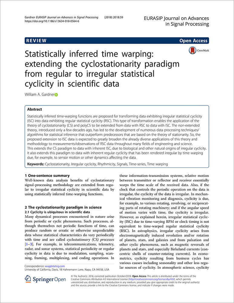
The reader is referred to the published article [JP65] shown immediately below for the details of the methodology for the analysis of Irregular Cyclicity. In addition, some stochastic process models for irregular cyclicity are introduced in [J39] and some alternative methods for dewarping are proposed. This latter contribution is discussed in the following section.

The following article is [J39]:
May 27, 2022
Summary
Two philosophically different approaches to the analysis of signals with imperfect cyclostationarity or imperfect poly-cyclostationarity of the autocorrelation function due to time-warping are compared in [4]. The first approach consists of directly estimating the time-warping function (or its inverse) in a manner that transforms data having an
empirical Empirical Data | noun Numerical quantities derived from observation or measurement in contrast to those derived from theory or logic alone. autocorrelation with irregular cyclicity into data having regular cyclicity [1]. The second approach consists of modeling the signal as a time-warped poly-cyclostationary stochastic Stochastic | adjective Involving random variables, as in stochastic process which is a time-indexed sequence of random variables. process, thereby providing a wide-sense probabilisticProbabilistic | noun Based on the theoretical concept of probability, e.g., a mathematical model of data comprised of probabilities of occurrence of specific data values. characterization–a time-varying probabilistic autocorrelation function–which is used to specify an estimator of the time-warping function that is intended to remove the impact of time-warping [3].
The objective of the methods considered is to restore to time-warped data exhibiting irregular cyclicity the regular cyclicity, called (poly-)cyclostationarity, that data exhibited prior to being time-warped. An important motive for de-warping data is to render the data amenable to signal processing techniques devised specifically for (poly-)cyclostationary signals. But in some applications, the primary motive may be to de-warp data that has been time-warped with an unknown warping function, and the presence of (poly-)cyclostationarity from the data source prior to that data becoming time warped is just happenstance that fortunately provides a means toward the dewarping end.
Time Warping of (Poly-)Cyclostationary Signals
Let be a wide-sense cyclostationary or poly-cyclostationary signal with periodically (or poly-periodically) time-varying autocorrelation
(1)
In (1), denotes optional complex conjugation, subscript
, and
, depending on
, is the countable set of (conjugate) cycle frequencies.
The expectation operator has two interpretations. It is the ensemble average operator in the classical stochastic approach or it is the poly-periodic component extraction operator in the fraction-of-time (FOT) probability approach. In both approaches, which are equivalent in the case of cycloergodicity, the cyclic autocorrelation function
can be estimated using a finite-time observation by the (conjugate) cyclic correlogram
(2)
In (2), is a realization of the stochastic process (with a slight abuse of notation) in the classical stochastic approach or the single function of time in the FOT approach.
Let be an asymptotically unbounded nondecreasing function. The time-warped version of
is given by
(3)
The time-warped signal is not poly-CS unless the time warping function
is an affine or a poly-periodic function.
In the following sections, two approaches are reviewed to estimate the time warping function or its inverse in order to de-warp to obtain an estimate of the underlying poly-CS signal. Once this estimate is obtained, cyclostationary signal processing techniques can be used.
Cyclostationarity Restoral
The first approach [1] consists of directly estimating the time-warping function (or its inverse
) in a manner that transforms the data
having an autocorrelation reflecting irregular cyclicity into data having regular cyclicity. Signals are modeled as single functions of time (FOT approach).
Specifically, assuming that exhibits cyclostationarity with at least one cycle frequency
, estimates
or
of
or
are determined such that, for the recovered signal
, the amplitude of the complex sine wave at frequency
contained in the second-order lag-product
is maximized.
Let
(4)
be a set of (not necessarily orthonormal) functions. Two procedures are proposed in [1]:
Procedure a) Consider the expansion
(5)
where and
, and maximize with respect to
the objective function
(6)
(7)
for some specific value of
. (Generalizations of
that include sums over
and/or
are possible.)
Procedure b) Consider the expansion
(8)
where , and maximize with respect to
the objective function
(9)
(10)
where (10) is obtained from (7) by the variable change and
(11)
The value of the vector or
that maximizes the corresponding objective function is taken as an estimate of the coefficient vector for the expansion of
or
. The maximization can be performed by a gradient-ascent algorithm, with starting points throughout a sufficiently fine grid.
In both approaches a) and b) data must be re-interpolated in order to evaluate the gradient of the objective function at every iteration of the iterative gradient-ascent search method. This is very time-consuming. However, for , method b) does not require data interpolation, and its implementation can be made very efficient. There are several important design parameters, which are discussed in [1].
Characterization and Warping Function Measurements
The second approach [3] consists of modeling the underlying signal as a time-warped poly-CS stochastic process, thereby providing a wide-sense probabilistic characterization of
in terms of the time-varying autocorrelation function. From this model, an estimator of
aimed at removing the impact of time warping is specified. From this estimate, an estimate of the autocorrelation function of the time-warped process is also obtained.
From (1) and (3), the (conjugate) autocorrelation of immediately follows:
(12)
A suitable second-order characterization can be obtained by observing that time-warped poly-cyclostationary signals are linear time-variant transformations of poly-cyclostationary signals. Thus, they can be modeled as oscillatory almost-cyclostationary (OACS) signals [2, Sec. 6].
Let us consider the warping function
(13)
(14)
In such a case, it can be shown that the autocorrelation (12) is closely approximated by
(15)
Two methods are proposed in [3] for estimating the function .
The first one considers the expansion
(16)
where , and provides estimates of the coefficients
by maximizing with respect to
the objective function
(17)
(18)
and is a set of values of
where
is significantly non zero. The maximization can be performed by a gradient ascent algorithm. The estimated coefficients are such that the additive-phase factor
in the expected lag-product of
(15) is compensated in (17) by using (18).
For the second method, let us define
(19)
with the impulse-response function of a low-pass filter with monolateral bandwidth
. Under the assumption that the spectral content of the modulated sine waves in (15) do not significantly overlap, and the low-pass filter extracts only one such sine wave, we have that
. Therefore,
can be estimated by
(20)
to within the unknown constant, where denotes the unwrapped phase. This method is also extended in [3] to the case where only a rough estimate of
is available.
De-Warping
Once the warping function or its inverse is estimated, the time-warped signal
can be de-warped in order to obtain an estimate
of the underlying poly-cyclostationary signal
. If this dewarping is sufficiently accurate, it renders
amenable to well known signal processing techniques for poly-cyclostationary signals (e.g., FRESH filtering).
If the estimate is obtained by the Procedure a) then the estimate of
is immediately obtained as
(21)
which would have already been calculated in (7). In contrast, if the estimate is available by the Procedure b) or by one of the two methods based on the OACS model, the estimate
should be obtained by inverting
.
In the case of , with
slowly varying, it can be shown that a useful estimate of
is [3]
(22)
provided that the estimation error is sufficiently small.
References
[1] W. A. Gardner, “Statistically inferred time warping: extending the cyclostationarity paradigm from regular to irregular statistical Statistical | adjective Of or having to do with Statistics, which are summary descriptions computed from finite sets of empirical data; not necessarily related to probability. cyclicity in scientific data,” EURASIP Journal on Advances in Signal Processing, vol. 2018, no. 1, p. 59, September 2018.
[2] A. Napolitano, “Cyclostationarity: Limits and generalizations,” Signal Processing, vol. 120, pp. 323–347, March 2016.
[3] A. Napolitano, “Time-warped almost-cyclostationary signals: Characterization and statistical function measurements,” IEEE Transactions on Signal Processing, vol. 65, no. 20, pp. 5526–5541, October 15 2017.
[4] A. Napolitano and W. A. Gardner, “Algorithms for analysis of signals with time-warped cyclostationarity,” in 50th Asilomar Conference on Signals, Systems, and Computers, Pacific Grove, California, November 6-9 2016.