The objective of this page 3 is to discuss the proper place in science and engineering of the fraction-of-time (FOT) probability model for time-series data, and to expose the resistance that this proposed paradigm shift has met with from those indoctrinated in the more abstract theory of Stochastic Processes, to the exclusion of the alternative FOT-probability theory. It is helpful to first consider the broader history of resistance to paradigm shifts in science and engineering. The viewer is therefore referred to Page 7, Discussion of the Detrimental Influence of Human Nature on Scientific Progress, as a prerequisite for putting this page 3 in perspective.
There are multiple independent contributions provided on this page in sections 3.2 – 3.6, all of which share a common purpose: to review the concept of Fraction-of-Time (FOT) probability, an alternative to the more widely taught stochastic process (or population-based probability), and to address the central argument put forth here that FOT probability, despite being highly relevant in many engineering and science applications, with clear advantages for specific purposes, is generally overlooked in academia in favor of stochastic process models. These contributions explain the core differences, highlight the historical reasons for the current situation, and argue for a more balanced approach in education and in practice. The contributions appear in reverse chronological order, with the most recent publication at the beginning. For this reason, the most efficient way to read them is to start with the first contribution and continue in reverse chronological order, skimming material that is a repeat from already read contributions, and focusing on different perspectives given and different emphases in the earlier contributions.
Main Themes
Paradigm Shift: This website page explains that a paradigm shift that would move teaching and practice from the stochastic process definition of probability to the FOT definition of probability, in fields involving time series analysis, was called for in 1987 and is still not happening! The thesis of the contributions provided on this page is that this proposed paradigm shift is still and will always be needed and support for this position is provided in the form of extensive and, it’s fair to say, even comprehensive, facts, comparative analysis, historical perspective, logic, and I would common sense. Although there are some technicalities that merit delving into, it is not difficult to see right at the outset what the advantages of FOT-Probability are. Although the first contribution, in Section 3.2, was the last to be written and can be considered to be a capstone on all that was written before, the earlier contributions that follow are partly unique and contain complementary perspectives and details.
Two Meanings of Probability: There are two fundamental ways of mathematically defining probability:
Stochastic Process (Population) Probability: This mathematical model is based on the idea of a “sample space,” which is a hypothesized (axiomatic) population of time functions from which samples can be randomly drawn. Probability is defined as an abstract function (a measure) of subsets (called events) within this space. This axiomatic approach is championed by mathematicians for certain theoretical developments. Including mathematical amenability to theorem proving, and non-empirical applicability outside of time series analysis. Other previously purported advantages of the stochastic process are challenged with sound argumentation.
Fraction-of-Time (FOT) Probability: This mathematical model is not axiomatically defined. Rather, it is computed from empirical time averages of prescribed measurement functions on a single time series of data (an empirical time function). Probability is defined as the fraction of time an event occurs over the lifetime of the function. There are two alternative theories here.
(1) Limit FOT-Probability. This is defined to be the limit, as averaging time conceptually/mathematically grows without bound (some would say “approaches infinity”, but nothing in the real-world approaches infinity, as argued in the field of Finitism). In this case, it is argued that all random effects in the average disappear in the limit (as they do when one takes an expected value of a stochastic process). This approach is championed for its elegance in application to real data, practicality, and direct relevance to single empirically observed time series of data; there is no assumption of an abstract population.
(2) 100% Empirical FOT-Probability. This is defined as described in (1) except that a finite averaging time is used. This approach is championed for being 100% empirical, requiring no abstract axioms, no assumed populations, no abstract limits, yet admitting a full probability theory for calculation and a corresponding completely empirical methodology that is more transparent than that for the stochastic process.
Succinct Comparison of FOT-Probability and the Stochastic Process:
Currently in scientific research, most time series analysts use methods that develop abstract models as in Option (1), from which real data behavior in the form of time-average statistics can possibly be mimicked by model-simulated data. The model can be used to perform abstract (data-free) probabilistic analysis of the simulated statistics as if they were the real time-average statistics from the real data. To illustrate that the theoretical results are realistic, they are compared with results from Monte Carlo simulations which try to mimic the model. This procedure is scientifically flawed because it is not based on the real world, with real data, and even though the model might fairly-well represent the real world in some ways (something that is not easily tested), it is still not actually the real world. When seeking to understand real physical phenomena, this is a critical flaw because, in real science, the model should come directly from the data; it should not be axiomatically posited. Moreover, when scientific experimentation produces only a single time series of data, it is non-parsimonious to use a model of a hypothetical population (ensemble) of time series in order to perform probabilistic analysis.
With option (2), the Fraction-of-Time probability method, the analyst uses, in a straightforward manner, only real data to produce a probabilistic analysis of the real statistics of the real data to gain insight into the source of the data that is being investigated, typically some phenomenon. The only obvious reason this might not be scientifically superior to the stochastic process method is that the real data may somehow be faulty or maybe there just isn’t enough of it to perform enough time-averaging. In either case, the scientist is likely faced with more serious challenges than choosing between two classes of models.
The ergodicity theorem and the law of large numbers from the theory of population-probability and statistics are cited by analysts to try to support the assumption that the model-simulated data does accurately represent the real data, but this argument is illogical because the mathematical results from this theorem and law concern only the abstract model, with no connection whatsoever to the real data.
Fortunately, dear reader, I understand the difficulty people have changing their minds about things. So, I have catered to this challenge in several ways. One is my attempt to make all the mathematical arguments fairly tutorial. A second is to gradually transition from succinct and directly-to-the-point arguments to longer, one might even say, drawn-out, arguments with considerable detail. In addition, following a set of published research journal papers, a detailed narrative including excerpts from a published debate on the issue addressed here is provided. This debate dates back 30 years to 1994-1995. The purpose of including this debate is to underscore the illogical nature of the resistance to this proposed paradigm shift with actual argumentation back and forth between the position taken here and the counter position that denies any advantage offered by the Fraction-of-Time definition of probability. It is my opinion that the counter argument is so weak and pitiful in its effort to support its position that it is embarrassing. Still this embarrassment is reprinted here to drive home the depth of illogical resistance to the proposed paradigm shift, which has sat mostly idle for almost 4 decades, arguably because of “nothing more than” the peculiarities of human behavior in the face of change. It is worthy of note that, to the best of my knowledge, no other debates or arguments of any flavor that oppose the proposed paradigm shift have been published since the original adoption of the stochastic process model about 75 years ago. Considering the case presented here, it is hard to imagine any basis for the absence of a paradigm shift other than inertia, a concept that captures Humanity’s natural resistance to change. This is, perhaps, one of the most salient reasons that science does not advance more quickly.
Call for Change in Education
One of the products of the argument presented here is the position that both types of probability are essential tools and a balanced education that includes both definitions is of crucial importance. To put it succinctly, I can find no good reason for university instructors in engineering and science to choose between introducing students exclusively to population probability or non-population probability. The position taken here calls for supplementing the standard stochastic process introduction with FOT probability, to enable students and, more importantly, graduates to choose the most appropriate model for the practical problems they encounter. The strong analogy between the two probability definitions enables efficient treatment in such a supplement, following standard treatment of stochastic processes. Although it might be argued that the stochastic process is generally more relevant than FOT-probability in engineering, this generalization overlooks the field of Investigative Engineering, which is akin to science for which the objective is to gain an understanding of natural phenomena through analysis of empirical measurements, not starting out by positing an abstract mathematical model.
Endorsements of the Call for Change
Section 3.2 below as well as some of the published papers presented below include verbatim quotations of giants in engineering and science, all of whom have passed since their endorsements of the paradigm shift called for here shortly following the appearance of the 1987 seminal book [Bk2], which introduced the first relatively complete theory of FOT-probability for stationary, cyclostationary, and almost cyclostationary time series, the latter two of which accommodate statistical cyclicity in time series data. The superlative credentials of these endorsement writers speak volumes about the merit of the proposed paradigm shift.
What does “probability & statistics” mean? These two terms are often used together, but they are two distinct entities. The field of Mathematical Statistics uses mathematical probability theory to model empirical statistics. But probability exists in its own right as an abstract mathematical theory and statistics exists in its own right as a collection of empirical methods for analyzing data. The blend of probability and statistics is a whole that is bigger than the sum of its parts, but those who forget that statistics are empirical and the stochastic-process definition of probability is mathematical are inviting confusion.
The picture of mathematical statistics comes into much better focus once the concept of the FOT alternative definition of probability is considered. The stark contrast between 100% empirical statistics (which get replaced with abstract sample paths of the assumed stochastic process in conventional mathematical statistics) and 100% abstract probability is done away with to differing extents, depending on which of Option (1) and Option (2) definitions of FOT-probability is considered. For Option (2), probability becomes 100% empirical, just like the statistics; for Option (1), probability retains some abstraction because it is based on the limit as averaging time grows without bound; however, it jettisons the abstraction of an assumed population of time series, which is particularly helpful for applications where there is only a single time-series record.
As an example of variations on an application where populations are, in one case, appropriate and, in another case, inappropriate, consider designing a digital communication system wanting the bit-error rate for a received signal over time to be less than 1 bit-decision error in 100 bit-decisions, on average over time. Here, we want the fraction of time the bit decision is in error for this signal to be less than 1/100, which is called the fraction-of-time (FOT) probability of a bit error. In another case, if we are producing a large number of communication systems and we want the number of systems that make bit-decision errors at any arbitrary time to be less than 1 in a 100, on average over the ensemble of systems, then we want the fraction of systems that make errors to be less than 1/100. This is the relative frequency of bit errors, and it converges as the communication-system ensemble size grows without bound to the relative-frequency (RF) probability of bit error which is, according to Kolmogorov’s Law of Large numbers, the stochastic probability of the bit-error event. This is a purely theoretical quantity in an abstract mathematical model of an ensemble of signals (one from each system) called a stochastic process.
These two probabilities are distinct and, in general, there is no reason to expect them to equal each other. Nevertheless, there is a weak link between the two that is established by the Ergodicity Theorem and the Law of Large Number, as explained in the following succinct comparison.
Ergodicity and the Law of Large Numbers
A source of confusion by some who invoke the ergodic hypothesis is thinking it is a hypothesis about the real data they are analyzing when, in fact, it is a hypothesis about the mathematical model they have adopted. Confusion surrounding the ergodic hypothesis can be avoided in many applications by first determining what is of primary interest in the application being studied: Is it the behavior of long-time averages or the behavior of large-ensemble averages? If it is the former, the analysist should simply adopt FOT probability (assuming sufficient data exists) and forget all about stochastic probability and the ergodic hypothesis.
As simple and self-evident as this truth is, some experts indoctrinated in the theory of stochastic processes have argued that FOT probability is an abomination that has no place in mathematical statistics (see subsequent section on the debate). The purpose of this Page 3 is to establish once and for all how absurd this extreme position is by addressing concerns about FOT probability that have been expressed in the past and extinguishing these concerns and associated claims that there is a controversy, through careful conceptualization, mathematical modeling, and straightforward discussion. As explained on this Page 3, there is no basis for controversy; there is simply a need to make a choice between two options for modeling probability in each application of interest.
For the Option (2) definition of probability, the concept of ergodicity is completely irrelevant: everything is empirical and there is no abstract stochastic process. However, for the Option (1) definition, the concept of ergodicity can be made relevant by complicating Option (1) by hypothesizing there is a population of time-series records. Then the two alternative types of probability, FOT and RF (relative frequency) can both be considered to be statistics—they can be computed from finite amounts of empirical data. They also can be interpreted as estimates of the limiting mathematical quantities, and they can exhibit some of the same properties as the mathematical quantities, but they are statistics, not probabilities. Moreover, the quantity that each converges to is just a number for a given set of statistics from any single execution of the underlying experiment (one experiment involves an infinitely long record of a time series, and the other involved an infinite set of time series records. These quantities are not mathematical models. But the collection of all such numbers obtained from all possible sets of statistics from hypothetical repeated trials of the underlying experiments (each trial involves an infinitely long record or an infinite ensemble) behave according to a probabilistic model. (This is definitely confusing because for the ensemble-average statistics, there is the assumption of an ensemble of ensembles—don’t blame me—I didn’t make up this stuff; the originators of the stochastic process did.) With this optional (assuming hypothetical repeated trials) perspective, the Ergodicity Theorem and the Law of large Numbers are both directly relevant for determining if these two limit probabilities equal each other (with probability equal to 1). (Personally, I don’t see how anyone could fall in love with the stochastic-process definition of probability with its requirement of a hypothetical ensemble of a hypothetical ensemble in order to probabilistically analyze population averages; but this requirement comes directly from the proof of the Law of Large Numbers.)
If It Ain’t Broke, Don’t Fix It
A grammarian’s version of this section title is “If it isn’t broken don’t attempt to fix it.” Regardless of how this is verbalized, the problem with how this way of thinking is often misapplied is that “it” IS often broken relative to what could be, but users are so accustomed to “it” that they don’t realize it could work much better.
Those who resist the proposed paradigm shift appear to abide by the philosophy described by this section title. Consider, as an example, the technology I used for preparing my doctoral dissertation in the early 1970s. I used an IBM Selectric typewriter and Snopake correction fluid (a fast-drying fluid that is opaque and as “white as the driven snow”), which enables the typist to paint over a mistake and then retype on the dried paint (beware of retyping before the paint is dry). I used this same technology for the first two books I wrote in the mid-1980s, after writing several drafts in longhand. It seemed acceptable at the time but, in comparison with the word processing technology I used to prepare this website, it is abundantly clear just how broken that technology was. Of course, adopting the superior word processing technology required the effort to first learn how to operate a personal computer. This learning “hump” that writers needed to get over resulted in many potential benefactors avoiding (actually only postponing) the chore of “coming up to speed” with PCs or Macs (Apple computers). The paradigm shift began for some upon the 1984 release of the first Apple Macintosh system, following the 1976 release of the first Apple computer, and for others it began with the 1989 release of the first Microsoft Word application for PCs. Others began jumping on board throughout the 1990s and by the turn of the Century this paradigm shift was well on its way. Today, we have electronic research journals for which new knowledge need never be recorded on paper. Thankfully someone decided a long time ago that the IBM Selectric Typewrite was indeed broken. The term word processing was actually created way back in 1950 by Ulrech Steinhilper, a German IBM typewriter sales executive with vision.
So it goes with many users of stochastic processes today: they have used this tool for years—since around 1950—and they see it as unbroken and they want no part of coming up to speed on a replacement tool that they believe isn’t needed, even though they do not yet understand this new tool. Unfortunately, ways of thinking are harder to change than is accepting new technology.
The cyclostationarity paradigm shift did not really take off until several years following the publication of the seminal 1987 book [Bk2]. It seems the same is going to be true for the FOT-Probability paradigm shift, with this website playing a role similar to that played by the 1987 book. Interestingly, that book attempted to initiate this shift as well as the shift to cyclostationarity 38 years ago. But apparently, the relearning hump for replacing stochastic processes was found to be too high for many.
As explained in this section, there are various choices to be made in deciding how best to present the more mathematical details of the theory of time-average probability, also called Non-Population Probability, and the choices made here are all based on pedagogy and a desire to accurately reflect the history of the subject to help newcomers understand what happened in the history of time-series analysis that led to the present predicament of living with a wrong choice.
The pedagogical considerations of interest are explained in the following discussion.

The macroscopic world that our five senses experience—sight, hearing, smell, taste and touch—is analog: forces, locations of objects, sounds, smells, temperature, and so on change continuously in time and space. Such things varying in time and space can be mathematically modeled as functions of continuous time and space variables, and calculus can be used to analyze these mathematical functions. For this reason, developing an intuitive real-world understanding of time-series analysis, and as an example spectral analysis of time-records of data from the physical world, requires that continuous-time models and mathematics of continua be used.
Unfortunately, this is at odds with the technology that has been developed in the form of computer applications and digital signal processing (DSP) hardware for carrying out numerical analysis, such as calculating spectra. This technology is based on discrete-time and discrete function-values, the numerical values of quantized and digitized time samples of various quantitative aspects of phenomena or of continuous-time and -amplitude measurements. Therefore, in order for engineers, scientists, statisticians, and others to design and/or use the available computer software tools and DSP Hardware for data analysis and processing at a deeper-than-superficial level, they must to some extent learn the discrete-time theory of the methods available—the algorithms implemented in computer software and DSP Hardware. The discreteness of the data values that this equipment processes can be ignored in the basic theory of statistical spectral analysis until the question of accuracy of the data representations subjected to analysis and processing arises. Then, the number of discrete-amplitude values used to represent each time sample of the original analog data, which determines the number of bits in a digital word representing a data value, becomes of prime importance as does the numbers of time samples per second. This discretization of time-series data values and time indices both affect the processing of data in undesirable ways, including spectral aliasing and nonlinear effects.
Consequently, essentially every treatment of the theory of spectral analysis and statistical spectral analysis available to today’s students of the subject presents a discrete-time theory. This theory must, in fact, be taught for obvious reasons but, from a pedagogical perspective, it is the Content Manager’s tenet that the discrete-time digital theory should be taught only after students have gained an intuitive real-world understanding of the principles of spectral analysis of continuous-time analog data, both statistical and non-statistical analysis. And this requires that the theory they learn be based on continuous-time mathematical models. This realization provides the motivation for the treatment presented at this website in which continuous-time time series data is used more frequently than discrete-time time series, though not exclusively.
Certainly, for non-superficial understanding of the use of digital technology for time-series analysis, the discrete-time theory must be learned. But for even deeper understanding of the link between the physical phenomena being studied and the analysis and processing parameters available to the user of digital technology, the continuous-time theory must also be learned. In fact, considering as an example the application of statistical spectral analysis, because of the additional layer of complexity introduced by the approximation of analog data with digital representations, which is not directly related to the principles of analog spectral analysis, an intuitive comprehension of the principles of spectral analysis, which are independent of the implementation technology, are more transparent and easier to grasp with the continuous-time theory, as demonstrated in [Bk4].
In the next Section, 3.2, the first self-contained published journal paper on the Fraction-of-Time Probability theory for cyclostationary and almost-cyclostationary time series is provided as a succinct basis for this entire page 3. Despite the passage of 34 years since its publication, it retains its value as a uniquely concise yet complete presentation of the basic theory of FOT-probability.
In Sections 3.3-3.7, five full-length research papers looking at the issue addressed on this page 3 from every conceivable angle and presenting in-depth perspectives based on mathematical analysis and empirical thinking are provided as a sound basis for the proposed paradigm shift from stochastic processes to the FOT-probability model.
In Section 3.3, a comprehensive argument taking into account all relevant perspectives that have occurred to the Author over decades of study is presented. The objective is to “leave no stone unturned” in this pursuit of truth about how best to perform probabilistic analysis in empirical science. Following this, subsequent sections each contain distinct published presentations of the relative pros and cons of the two competing definitions of probability.
In Section 3.4, the paper “On Cycloergodicity” dives deeply into the ergodicity quagmire of stochastic process theory, extending and generalizing tradition ergodicity theory from stationary and asymptotically mean stationary stochastic processes to cyclostationary and asymptotically mean cyclostationary processes and to almost cyclostationary and asymptotically mean almost cyclostationary processes. After exposing startling issues for unsuspecting users that arise from non-cycloergodic stochastic process models and then exposing the substantial mathematical challenge presented to time series analysts by the need to validate their use of the cycloergodic hypothesis, the thesis of this page 3 is introduced and various arguments in support of the proposed paradigm shift are given.
These two papers in Sections 3.3, 3.4 together present “the last word” on this topic. Yet, there are three more earlier publications that follow in Sections 3.5-3.7, with complementary facts, perspectives, and arguments that support the first two papers.
Before proceeding to these in-depth arguments in support of the proposed paradigm shift, a historical listing of the most well-known contributors to the probabilistic modeling of time series is provided. The history of the development of time-series analysis can be partitioned into the earlier empirically driven work focused on primarily methodology, which extended over a period of about 300 years, and the later but overlapping mathematically driven work, in which the theory of stochastic processes surfaced, and ran its course of primary development of the basics with regard to time series analysis in about 50 years. The mathematically driven development of stochastic processes has continued beyond that initial period, but has centered on primarily nonstationary processes, rather than primarily stationary processes. The development of time series analysis theory and methodology for cyclostationary and related stochastic processes and their non-stochastic time-series counterparts came along later during the latter half of the 20th century and extends to the present.
As can be seen from these two lists, the stochastic process is the newcomer, which has overshadowed hundreds of years of preceding empirical work. As shown at this page 3, it is a mistake to think that the empirical objectives of 300 years’ worth of work are better met by the newcomer. It is argued herein that this newcomer serves a distinct purpose, which has largely ignored empiricism and therefore the bulk of applications of probability in the sciences. Thus, the proposed paradigm shift is not the product of an undisciplined upstart, as some may think. Rather, it is the product of a deep respect for the ubiquitous analytical needs of science, which is inherently an empirical discipline in which axiomatically defined models as a basis for empirical analysis are mostly out of place.
Mathematically Driven Development of Probability Spaces and Stochastic Processes as the Originally Preferred Conceptual/Mathematical Basis for Time Series Analysis (1900-1950)
Empirically Driven Development of Time-Series Analysis Methodology (1650-1950)
The following article, FRACTION-OF-TIME PROBABILITY FOR TIME-SERIES THAT EXHIBIT CYCLOSTATIONARITY, Signal Processing, Vol. 23, No. 3, pp. 273-292, by William A Gardner and William A Brown [JP34], was published in 1991, 5 years after this novel probability theory was introduced in the book [Bk2]. Thirty years hence, this article remains the single most complete and easy-to-read accounting of this probability theory aimed at a readership of statistical time-series analysis practitioners. For this reason, it is incorporated here as part of this Page 3, as an encouragement to readers to make this their first detailed encounter with this novel probability theory. In comparison with other worthy sources on this theory, including primarily the originating book [Bk2], the 2006 survey paper [JP64], the 2006 development of a measure-theory foundation [J24], and the most recent and most comprehensive treatment of cyclostationarity in general, the 2019 book [B2], this treatment is both concise and quite complete.
The above concise paper is based on the seminal 1987 book [Bk2]. Following are some quotations reflecting the reaction of leaders in the field to this book when it first came out.
The renowned researcher and author of over 20 books, Enders A. Robinson, wrote the following about the book:
“Professor Gardner has the ability to impart a fresh approach to many difficult problems. . . . His general approach is to go back to the basic foundations and lay a new framework. This gives him a way to circumvent many of the stumbling blocks confronted by other workers . . . he has discovered many avenues of approach which were either not known or neglected in the past. In this way his work more resembles some of the outstanding mathematicians and engineers of the past. . . . William’s success in the approach shows the strength of his engineering insight. He has been able to solve problems that others have left as being too difficult.”
Further to this, Robinson wrote a strongly supportive 1990 review of this book that includes the following excerpt:
“This book can be highly recommended to the engineering profession. Instead of struggling with many unnecessary concepts from abstract probability theory, most engineers would prefer to use methods that are based upon the available data. This highly readable book gives a consistent approach for carrying out this task. In this work Professor Gardner has made a significant contribution to statistical spectral analysis, one that would please the early pioneers of spectral theory and especially Norbert Wiener.”
Similarly, the following quotation from Professor Ronald N. Bracewell, 1994 recipient of the Institute of Electrical and Electronics Engineers’ Heinrich Hertz medal for pioneering work in antenna aperture synthesis and image reconstruction as applied to radio astronomy and to computer-assisted tomography, taken from his Foreword to the 1987 book introducing FOT-Probability theory [Bk2], makes essentially the same point that Robinson makes:
“If we are to go beyond pure mathematical deduction and make advances in the realm of phenomena, theory should start from the data. To do otherwise risks failure to discover that which is not built into the model . . . Professor Gardner’s book demonstrates a consistent approach from data, those things which in fact are given, and shows that analysis need not proceed from assumed probability distributions or random processes. This is a healthy approach and one that can be recommended to any reader.”
As another example,Dr. Akiva Yaglom, Mathematician and Physicist, USSR Academy of Sciences, wrote in his review of the Book published in Theory of Probability and Its Applications:
“It is important . . . that until Gardner’s . . . book was published there was no attempt to present the modern spectral analysis of random processes consistently in language that uses only time-averaging rather than averaging over the statistical ensemble of realizations [of a stochastic process] . . . Professor Gardner’s book is a valuable addition to the literature”
A fourth example is the following succinct enthusiastic remark given by Professor James L. Massey, information theorist and cryptographer, Professor of Digital Technology at ETH Zurich, in a prepublication book review in 1986:
“I admire the scholarship of this book and its radical departure from the stochastic process bandwagon of the past 40 years.”
As a final example, Professor Thomas Kailath of Stanford University, member of the National Academy of Engineering, the US National Academy of Sciences, the American Academy of Arts and Sciences, the Indian National Academy of Engineering, and the Silicon Valley Engineering Hall of Fame, wrote the following about the 1987 book:
“It is always hard to go against the established order, but I am sure that the book will have a considerable impact. It will be a definitive text on spectral analysis.” — Professor Thomas Kailath.”
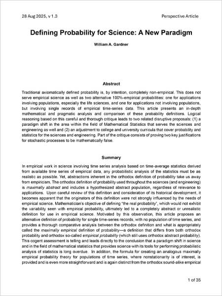
In empirical work in science involving time series analysis based on time-average statistics derived from available time series of empirical data, any probabilistic analysis of the statistics must be as realistic as possible. Yet, abstractions inherent in the orthodox definition of probability take us away from empiricism. The orthodox definition of probability used throughout the sciences (and engineering) is maximally abstract and includes a hypothesized abstract population, regardless of relevance to applications. Upon careful review of this definition and consideration of its historical development, it becomes apparent that the originators of this definition were not strongly influenced by the needs of empirical science. Mathematician’s objective of defining “the real probability”, which would not exhibit the variability seen with empirical probability, ultimately led to a completely abstract or unrealistic definition for use in empirical science. Motivated by this observation, the following article proposes an alternative definition of probability for single time-series records, with no population of time series, and provides a thorough comparative analysis between the orthodox definition and what is appropriately called the maximally empirical definition of probability—a definition that differs from both orthodox probability and orthodox so-called empirical probability (which still uses orthodox abstract probability). This cogent assessment is telling and leads directly to the conclusion that a paradigm shift in science and in the field of mathematical statistics that provides science with its tools for performing probabilistic analysis of statistics is long overdue. In addition, the formula for creating an analogous maximally empirical probability theory for populations of time series, where nonstationarity is of interest, is provided and is even more straightforward and is again distinct from the orthodox sound-alike empirical probability. Together, these two theories provide for both sciences not involving populations and the life sciences which typically do involve populations.
The following article is an unpublished treatise that is planned to be either replaced by or complemented with another treatise that provides additional insight into the history of the issue of choosing between stochastic process models of populations of functions and non-stochastic (also called stochastic-free) probabilistic models of individual functions. Specifically, this additional treatise presently (December 2025) in preparation for publication in 2026 is tentatively entitled “Modern Expanded Generalized Harmonic Analysis in Communications Engineering: An Example of Mathematical Pluralism” and is tentatively planned for submittal to the Journal of Fourier Analysis and Applications. This treatise includes a more in-depth treatment of the history surrounding Norbert Wiener’s philosophy of mathematical pluralism that explains his contributions to and use of both stochastic and stochastic-free models of functions as tools for probabilistic and/or statistical analysis. More specifically, these two models are based on two alternative definitions of probability. Accordingly, this late-coming additional treatise is the result of the recent discovery of a 31-year-old extensive discussion of Wiener’s use of both types of models and his philosophy supporting this mathematical pluralism in contrast to the century-long dominance of orthodox non-pluralistic mathematics, called foundational mathematics that began falling out of favor at the turn of the century and is presently receiving considerable attention in the mathematics literature, cf. [ https://mally.stanford.edu/Papers/math-pluralism.pdf ] and [https://assets.cambridge.org/97810095/00968/frontmatter/9781009500968_frontmatter.pdf ].
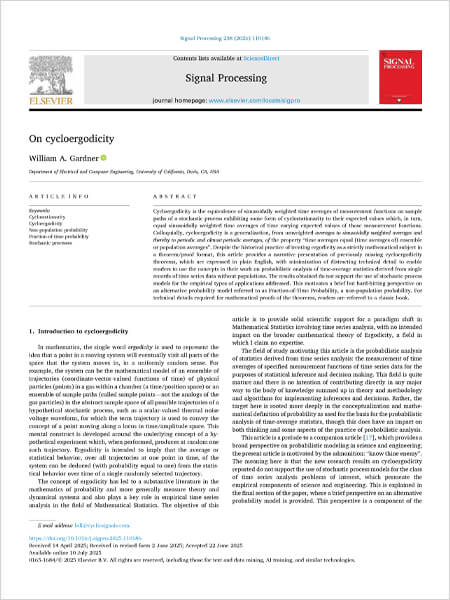
In the paper in this section, cycloergodicity theorems identified as missing for 40 years are introduced, necessary and sufficient tests for determining cycloergodicity are identified, new measure-theory ingredients required by cycloergodicity theorems introduced, practical Irrelevance of theorems to data analysis without real populations is explained, and stochastic process models when there are no real populations are explained to be nonscientific. Cycloergodicity is the equivalence of sinusoidally weighted time averages of measurement functions on sample paths of a stochastic process exhibiting some form of cyclostationarity to their expected values which, in turn, equal sinusoidally weighted time averages of time varying expected values of those measurement functions. Colloquially, cycloergodicity is a generalization, from unweighted averages to sinusoidally weighted averages and thereby to periodic and almost periodic averages, of the property “time averages equal (time averages of) ensemble or population averages”. Despite the historical practice of treating ergodicity as a strictly mathematical subject in a theorem/proof format, this article provides a narrative presentation of previously missing cycloergodicity theorems, which are expressed in plain English, with minimization of distracting technical detail to enable readers to use the concepts in their work on probabilistic analysis of time-average statistics derived from single records of time series data without populations. The results obtained do not support the use of stochastic process models for the empirical types of applications addressed. This motivates a brief but hard-hitting perspective on an alternative probability model referred to as Fraction-of-Time Probability, a non-population probability. For technical details required for mathematical proofs of the theorems, readers are referred to a classic book.
For purposes of developing intuition and possibly deeper understanding regarding the FOT-Probability model introduced in Section 3.2, the reader is referred to the following article which contrasts it with the conventional stochastic process model. The standard theoretical foundation for statistical processing of persistent signals, whether they are signals representing sound and vibration, or radio-frequency transmission, or time series of measurements on just about any persistent phenomenon, is presently the discrete-time and continuous-time Kolmogorov stochastic process models and especially, but not exclusively, strongly ergodic and cycloergodic Kolmogorov stochastic process models satisfying the axiom of relative measurability, which guarantees that limits of time averages on functions of sample paths exist. After a brief discussion exposing drawbacks of these generic models for many applications in statistical signal processing, particularly those involving empirical data, an alternative stochastic process model is proposed for statistically stationary signals, and a complementary model for statistically cyclostationary signals also is proposed. For these alternative models, defined first in terms of a parsimonious construction of their samples spaces, their cumulative probability distribution functions (CDFs) are derived from Fraction-of-Time (FOT) Probability calculations on a single member of the sample space, defined in terms of the Kac-Steinhaus relative measure on the Real line, and they are then shown to be valid CDFs over the entire sample space of the process. If all such finite-dimensional CDFs are specified, then this corresponds to a complete probabilistic model for the alternative stochastic process—equivalent to the specification of a probability measure defined directly on the sample space. The motivating difference between Kolmogorov’s model and this alternative parsimonious model is that the alternative is derived from empirical data, at least in principle. It is not posited in an abstract axiomatic manner that typically leads to a number of conceptually confusing and often unanswerable questions about the behavior of the sample paths in the model. These preferred alternative models are also complemented with another empirically derived model, this one for poly-cyclostationary signals that exhibit multiple incommensurate periods of cyclostationarity, but this model does not have an associated sample space for reasons explained herein.
For manmade signals, such as those typically encountered in communications and signals intelligence systems, applied R&D in statistical signal processing is typically based on formulaic signal models specified by explicit mathematical formulas containing deterministic functions of time, and individual random variables, sequences of independent random variables, and standard stochastic processes, such as stationary Gaussian or uniformly distributed processes. In such cases, the user can sometimes derive mathematical properties that will be useful in mathematical analysis, such as derivations of solutions to statistical inference and decision-making optimization problems. But this is often beyond the scope of specific applications and, as a result, assumptions about the models are typically made without justification. Sometimes, very broad but unproven justifications are used. For example, the analyst may assume a specified model satisfies the axiomatic definition of a Kolmogorov stochastic process. Examples of properties of the probability measure defining a Kolmogorov process include sigma-additivity (additivity of countably infinite numbers of terms), sigma-linearity (linearity of an operator applied to a linear combination of a countably infinite number of terms), and joint-measurability of two or more processes, which is necessary for the existence of joint probability density functions. These properties of a specific model are often not verifiable, despite their being assumed to hold. While this is common practice, it does not follow the scientific method that should guide all science and engineering.
Hidden periodicities in science data have long been a popular topic of investigation. The popularity stems from the fact that detecting and characterizing periodicities can provide a means for extracting information from science data—information that might not otherwise be accessible. In other words, periodicities in data can be exploited for the purposes of statistical inference and decision making. The long history of this topic is briefly reviewed with heavy reference to a historical essay on the topic by H.O.A. Wold, written more than half a century ago, following which the treatise focuses on a paradigm shifting advance in theory and methodology for characterizing hidden periodicities that was initiated by the second author in the mid-1980s and further advanced by both authors since then, including a plethora of algorithms for performing the needed computations in applications. The data models this theory is based on are generally called cyclostationary but include variations that are labeled with modifiers like wide-sense, strict sense, n-th order for n = 1, 2, 3,…, almost, poly, and irregular. The theory is probabilistic, but is intentionally not based on stochastic processes which, it is argued, are inappropriate for many, if not most, applications. The basis used is Fraction-of-Time (FOT) Probability. The concept, theory, and methodology of FOT Probability is itself a major paradigm shift, also initiated by the second Author more than half a century ago, and it is an integral part of the (preferred) non-stochastic theory of cyclostationarity. Since the birth of this topic, both authors have continued to advance these paradigm shifts, including further development of theory, associated methodology, and computational algorithms. The most advanced of the concepts described (viz., irregular poly-cyclostationarity) is illustrated with an application of the associated algorithms to science data consisting of time series of Sunspot numbers containing approximately 75,000 daily measurements representing a period of about 200 years. The results include the first methodical characterization of the irregularity of the poly-periodicity hidden in the data.
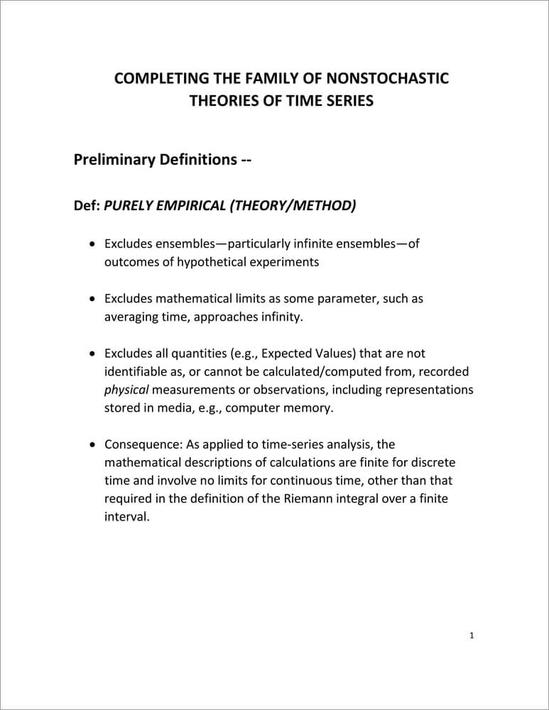
Statistical metrics for time series such as mean, bias, variance, coefficient of variation, covariance, and correlation coefficient can be defined using finite-time averages as replacements for expected values in well-known probabilistic metrics. These statistical metrics also can be arrived at from nothing more than a little thought, without any reference to probability or expected value. In fact, many of these statistical metrics were in use long before the probabilistic theory of stochastic processes was developed.
In the book [Bk2], such non-probabilistic statistical metrics are used for statistical spectral analysis. The resultant theory for understanding how to perform and study statistical spectral analysis is the lowest level in a hierarchy of non-stochastic theories of statistical spectral analysis and, more generally, time-series analysis. This level is referred to as the purely empirical non-probabilistic theory. It is quite adequate for many applications.
The next level up in the hierarchy is referred to as the purely empirical FOT-probabilistic theory, where FOT stands for Fraction-of-Time. The model upon which this theory is based is introduced in the presentation below. The third and highest level in the hierarchy is referred to as the non-stochastic FOT-probabilistic theory. This theory is fully developed in the book [Bk2]. The model is an asymptote of the model for the Finite-Time Theory described below. This asymptotic model can be approached as closely as one desires with the Finite-Time Model if enough time series data is available, but it cannot be reached exactly and still be empirical.
In subsection 3.8.2, the terms purely empirical, probabilistic, and non-stochastic are defined and the three individual levels of the hierarchy are defined and illustrated. The following material was mostly presented at the 2021 On-Line Grodek Conference on Cyclostationarity, but it is an improved version of that presentation.
Section 3.8 is concluded with a brief derivation in subsection 3.8.3 illustrating how the finite-time cyclostationary and poly-cyclostationary expectation operators are defined for finite segments of data, and another brief illustration in subsection 3.84 of how non-probabilistic expectation operators on finite data segments are defined and an explanation of the relationship between these and signal subspace methods of statistical inference. Both concepts use projections that are more general than those which function as constant-component extraction operators and periodic component extraction operators, both of which are probabilistic expectations.
The presentation slides presented immediately below address the mathematical foundation and framework, developed by the WCM, for statistical time-series analysis based on statistical functions such as correlations, higher-order moments, and cumulative probability distributions, without involving the abstract mathematical model of a stochastic process. The purpose is to facilitate conceptualization and practical application. The application addressed is statistical spectral correlation analysis.
The process by which the models of CS and Poly-CS time series are modified to render them applicable to data on finite-time intervals instead of infinite-time intervals is explained immediately below and supported with mathematical definitions.

The topic for this page is addressed immediately below:

This section reproduces a published debate on the pros and cons of the two alternatives for modeling random signals: The stochastic process and the FOT-Probability model. Unfortunately—as good debates go—the arguments against the FOT probability alternative are shallow, unconvincing, and in places erroneous. One can take this as an indication that opponents of FOT Probability simply do not have a strong position to argue from.
The 1987 book, Statistical Spectral Analysis: A Nonprobabilistic Theory, argues for more judicious use of the modern stochastic-process-model (arising from the work of mathematicians in the 1930s, such as Khinchin, Kolmogorov, and others) instead of the more realistic predecessor: the time-series model first developed mathematically by Norbert Wiener in 1930 (see also page 59 of Wiener 1949, written in 1942, regarding the historical relationship between his and Kolmogorov’s approaches), that was briefly revisited in the 1960s by engineers before it was buried by mathematicians. The brief tongue-in-cheek essay Ensembles in Wonderland, published in IEEE Signal Processing Magazine, AP Forum, 1994 and reproduced below, is an attempt at satirizing the outrage typified by narrow-minded thinkers exemplified by two outspoken skeptics, Neil Gerr and Melvin Hinich, who wrote scathing remarks and a book review characterizing this book as utter nonsense. (Page 7.6 offers an explanation for the behavior of these two naysayers in terms of weak right-brain thinking.)
But first, let us consider the parallel to the book Alice in Wonderland; the following is comprised of excerpts taken from https://en.wikipedia.org/wiki/Alice’s_Adventures_in_Wonderland : Martin Gardner and other scholars have shown the book Alice in Wonderland [written by Lutwidge Dodgson under the pseudonym Lewis Carroll] to be filled with many parodies of Victorian popular culture. Since Carroll was a mathematician at Christ Church, it has been argued that there are many references and mathematical concepts in both this story and his later story Through the Looking Glass; examples include what have been suggested to be illustrations of the concept of a limit, number bases and positional numeral systems, the converse relation in logic, and the ring of integers modulo a specific integer. Deep abstraction of concepts, such as non-Euclidean geometry, abstract algebra, and the beginnings of mathematical logic, was taking over mathematics at the time Alice in Wonderland was being written (the 1860s). Literary scholar Melanie Bayley asserted in the magazine New Scientist that Alice in Wonderland in its final form was written as a scathing satire on new modern mathematics that was emerging in the mid-19th century.
Today, Dodgson’s satire appears to be backward looking because, after all, there are strong arguments that modern mathematics has triumphed. Coming back to the topic of interest here, stochastic processes also have triumphed in terms of being wholly adopted in mathematics and science and engineering, except for a relatively small contingent of empirically-minded scientists and engineers. Yet, recent mathematical arguments, described in tutorial fashion on pages 3.2.and 3.3 and further supported with references cited there, provide a sound logical basis for reversing this outcome, especially when the overwhelming evidence of practical, pragmatic, pedagogic, and overarching conceptual advantages provided in the 1987 book and expanded on pages 3.2 and 3.3 here, is considered. The present dominance of the more abstract and less realistic stochastic process theory might be viewed as an example of the pitfalls of what has become known as groupthink or the inertia of human nature that resists changes in thinking, which is discussed in considerable detail based on numerous historical sources on Page 7.
Before presenting the several letters comprising the debate, including the standalone article “Ensembles in Wonderland”, the final letter to SP Forum in the debate is reproduced here first to provide hindsight, especially for interpreting “Ensembles in Wonderland”. The bracketed text, e.g., [text], below was added to the published debate specifically for this book to enhance clarity.
July 2, 1995 (published in Nov 1995)
To the Editor:
Introduction
This is my final letter to SP Forum in the debate initiated by Mr. Melvin Hinich’s challenge to the resolution made in the book [1], and carried on by Mr. Neil Gerr through his letters to SP Forum.
In this letter, I supplement my previous remarks aimed at clarifying the precariousness of Hinich’s and Gerr’s position by explaining the link between my argument in favor of the utility of fraction-of-time (FOT) probability and the subject of a plenary lecture delivered at ICASSP ’94. In the process of discussing this link I hope to continue the progress made in my previous two letters in discrediting the naysayers and thereby moving toward broader acceptance of the resolution that was made and argued for in [1] and is currently being challenged. My continuing approach is to show that the position taken by the opposition–that the fraction-of-time probability concept and the corresponding time-average framework for statistical signal processing theory and method have nothing to offer in addition to the concept of probability associated with ensembles and the corresponding stochastic process framework–simply cannot be defended if argument is to be based on fact and logic.
David J. Thomson’s Transcontinental Waveguide Problem
To illustrate that the stochastic-process conceptual framework is often applied to physical situations where the time-average framework is a more natural choice, I have chosen an example from D. J. Thomson’s recent plenary lecture on the project that gave birth to the multiple-window method of spectral analysis [2]. The project that was initiated back in the mid-1960s was to study the feasibility of a transcontinental millimeter waveguide for a telecommunications transmission system potentially targeted for introduction in the mid-1980s. It was found that accumulated attenuation of a signal propagating along a circular waveguide was directly dependent on the spectrum of the series, indexed by distance, of the erratic diameters of the waveguide. So, the problem that Thomson tackled was that of estimating the spectrum for the more than 4,000-mile-long distance-series using a relatively small segment of this series that was broken into a number of 30-foot long subsegments. (It would take more than 700,000 such 30-foot sections to span 4,000 miles.) The spectrum had a dynamic range of over 100 dB and contained many periodic components, indicating the unusual challenge faced by Thomson.
When a signal travels down a waveguide (at the speed of light) it encounters the distance-series [consisting of the distances traveled as time progresses]. Because of the constant velocity, the distance-series is equivalent to a time-series. Similarly, the series of diameters that is measured for purposes of analysis is—due to the constant effective velocity of the measurement device—equivalent to a time-series [of measurements]. So, here we have a problem where there is one and only one long time-series of interest (which is equivalent to a distance-series)—there is no ensemble of long series over which average characteristics are of interest and, therefore, there is no obvious reason to introduce the concept of a stochastic process. That is, in the physical problem being investigated, there was no desire to build an ensemble of transcontinental waveguides. Only one (if any at all) was to be built, and it was the spectral density of distance-averaged (time-averaged) power of the single long distance-series (time-series) that was to be estimated, using a relatively short segment, not the spectral density of ensemble-averaged power. Similarly, if one wanted to analytically characterize the average behavior of the spectral density estimate (the estimator mean) it was the average of a sliding estimator over distance (time), not the average over some hypothetical ensemble, that was of interest. Likewise, to characterize the variability of the estimator, it was the distance-average squared deviation of the sliding estimator about its distance-average value (the estimator variance) that was of interest, not the variance over an ensemble. The only apparent reason for introducing a stochastic process model with its associated ensemble, instead of a time-series model, is that one might have been trained to think about spectral analysis of erratic data only in terms of such a conceptual artifice and might, therefore, have been unaware of the fact that one could think in terms of a more suitable alternative that is based entirely on the concept of time averaging over the single time-series. (Although it is true that the time-series segments obtained from multiple 30 ft. sections of waveguide could be thought of as independent random samples from a population, this still does not motivate the concept of an ensemble of infinitely long time-series–a stationary stochastic process. The fact remains that, physically, the 30-foot sections represent subsegments of one long time-series in the communications system concept that was being studied.) [And even if Mr. Thomson was aware of the fact that one could conceptualize the problem entirely in terms of time averages, he had good reason to fear that this approach would be off-putting to his readers all of whom were likely indoctrinated only in statistical spectral analysis theory couched in terms of stochastic processes—an unfortunate situation].
It is obvious in this example that there is no advantage to introducing the irrelevant abstraction of a stochastic process (the model adopted by Thomson) except to accommodate lack of familiarity with alternatives. Yet Gerr turns this around and says there is no obvious advantage to using the time-average framework. Somehow, he does not recognize the mental gyrations required to force this and other physical problems into the stochastic process framework.
Gerr’s Letter
Having explained the link between my argument in favor of the utility of FOT probability and Thomson’s work, let us return to Gerr’s letter. Mr. Gerr, in discussing what he refers to as “a battle of philosophies,” states that I have erred in likening skeptics to religious fanatics. But in the same paragraph we find him defensively trying to convince his readers that the “statistical/probabilistic paradigm” has not “run out of gas” when no one has even suggested that it has. No one, to my knowledge, is trying to make blanket negative statements about the value of what is obviously a conceptual tool of tremendous importance (probability) and no one is trying to denigrate statistical concepts and methods. It is only being explained that interpreting probability in terms of the fraction-of-time of occurrence of an event is a useful concept in some applications. To argue, as Mr. Gerr does again in the same paragraph, that in general this concept “has no obvious advantages” and using it is “like building a house without power tools: it can certainly be done, but to what end?” is, as I stated in my previous letter, to behave like a religious fanatic — one who believes there can be only One True Religion. This is a very untenable position in scientific research.
As I have also pointed out in my previous letter, Mr. Gerr is not at all careful in his thinking. To illustrate his lack of care, I point out that Gerr’s statement “Professor Gardner has chosen to work within the context of an alternative paradigm [fraction-of-time probability]”, and the implications of this statement in Gerr’s following remarks, completely ignore the facts that I have written entire books and many papers within the stochastic process framework, that I teach this subject to my students, and that I have always extolled its benefits where appropriate. If Mr. Gerr believes in set theory and logic, then he would see that I cannot be “within” paradigm A and also within paradigm B unless A and B are not mutually exclusive. But he insists on making them mutually exclusive, as illustrated in the statement “From my perspective, developing signal processing results using the fraction-of-time approach (and not probability/statistics) … .” (The parenthetical remark in this quotation is part of Mr. Gerr’s statement.) Why does Mr. Gerr continue to deny that the fraction-of-time approach involves both probability and statistics?
Another example of the lack of care in Mr. Gerr’s thinking is the convoluted logic that leads him to conclude “Thus, spectral smoothing of the biperiodogram is to be preferred when little is known of the signal a priori.” As I stated in my previous letter, it is mathematically proven* in [1] that the frequency smoothing and time averaging methods yield approximately the same result. Gerr has given us no basis for arguing that one is superior to the other and yet he continues to try to make such an argument. And what does this have to do with the utility of the fraction-of-time concept anyway? These are data processing methods; they do not belong to one or another conceptual framework.
To further demonstrate the indefensibility of Gerr’s claim that the fraction-of-time probability concept has “no obvious advantages,” I cite two more examples to supplement the advantage of avoiding “unnecessary mental gyrations” that was illustrated using Thomson’s waveguide problem. The first example stems from the fact that the fundamental equivalence between time averaging and frequency smoothing referred to above was first derived by using the fraction-of-time conceptual framework [1]. If there is no conceptual advantage to this framework, why wasn’t such a fundamental result derived during the half century of research based on stochastic processes that preceded [1]? The second example is taken from the first attempt to develop a theory of higher-order cyclostationarity for the conceptualization and solution of problems in communication system design. In [3], it is shown that a fundamental inquiry into the nature of communication signals subjected to nonlinear transformations led naturally to the fraction-of-time probability concept and to a derivation of the cumulant as the solution to a practically motivated problem. This is, to my knowledge, the first derivation of the cumulant. In all other work, which is based on stochastic processes (or non-fraction-of-time probability) and which dates back to the turn of the century, cumulants are defined, by analogy with moments, to be coefficients in an infinite series expansion of a transformation of the probability density function (the characteristic function), which has some useful properties. If there is no conceptual advantage to the fraction-of-time framework, why wasn’t the cumulant derived as the solution to the above-mentioned practical problem or some other practical problem using the orthodox stochastic-probability framework?
Conclusion
Since no one in the preceding year has entered the debate to indicate that they have new arguments for or against the philosophy and corresponding theory and methodology presented in [1], it seems fair to proclaim the debate closed. The readers may decide for themselves whether the resolution put forth in [1] was defeated or was upheld.
But regarding the skeptics, I sign off with a humorous anecdote:
When Mr. Fulton first showed off his new invention, the steamboat, skeptics were crowded on the bank, yelling ‘It’ll never start, it’ll never start.’
It did. It got going with a lot of clanking and groaning and, as it made its way down the river, the skeptics were quiet.
For one minute.
Then they started shouting. ‘It’ll never stop, it’ll never stop.’
— William A. Gardner
* A more detailed and tutorial proof of this fundamental equivalence is given in the article “The history and the equivalence of two methods of spectral analysis,” Signal Processing Magazine, July 1996, No.4, pp.20 – 23, which is copied into the Appendix farther down this Page.
References
Excerpts from earlier versions of above letter to the editor before it was condensed for publication:
April 15, 1995
Introduction
In this, my final letter to SP Forum in the debate initiated by Mr. Melvin Hinich’s challenge to the resolution made in the book [1], I shall begin by addressing two remarks in the opening paragraph of Mr. Neil Gerr’s last letter (in March 1995 SP Forum). In the first remark, Mr. Gerr suggests that the “bumps and bruises” he sustained by venturing into the “battle” [debate] were to be expected. But I think that such injuries could have been avoided if he had all the relevant information at hand before deciding to enter the debate. This reminds me of a story I recently heard:
Georgios and Melvin liked to hunt. Hearing about the big moose up north, they went to the wilds of Canada to hunt. They had hunted for a week, and each had bagged a huge moose. When their pilot Neil landed on the lake to take them out of the wilderness, he saw their gear and the two moose. He said, “I can’t fly out of here with you, your gear, and both moose.”
“Why not?” Georgios asked.
“Because the load will be too heavy. The plane won’t be able to take off.”
They argued for a few minutes, and then Melvin said, “I don’t understand. Last year, each of us had a moose, and the pilot loaded everything.”
“Well,” said Neil, “I guess if you did it last year, I can do it too.”
So, they loaded the plane. It moved slowly across the lake and rose toward the mountain ahead. Alas, it was too heavy and crashed into the mountain side. No one was seriously hurt and, as they crawled out of the wreckage in a daze, the bumped and bruised Neil asked, “Where are we?”
Melvin and Georgios surveyed the scene and answered, “Oh, about a mile farther than we got last year.”
If Mr. Gerr had read the book [1] and put forth an appropriate level of effort to understand what it was telling him, he would have questioned Mr. Hinich’s book review and would have seen that the course he was about to steer together with the excess baggage he was about to take on made a crash inevitable.
A friend of mine recently offered me some advice regarding my participation in this debate. “Why challenge the status quo”, he said, “when everybody seems happy with the way things are.” My feeling about this is summed up in the following anecdote:
“Many years ago, a large American shoe manufacturer sent two sales reps out to different parts of the Australian outback to see if they could drum up some business among the aborigines. Sometime later, the company received telegrams from both agents.
The first one said. ‘No business. Natives don’t wear shoes.’
The second one said, ‘Great opportunity here–natives don’t wear shoes.'”
Another friend asked “why spend your time on this [debate] when you could be solving important problems.” I think Albert Einstein answered that question when he wrote:
“The mere formulation of a problem is far more essential than its solution, which may be merely a matter of mathematical or experimental skills. To raise new questions, new possibilities, to regard old problems from a new angle requires creative imagination and marks real advances in science”
This underscores my belief that we are overemphasizing “engineering training” in our university curricula at the expense of “engineering science.” It is this belief that motivates my participation in this debate. Instead of plodding along in our research and teaching with the same old stochastic process model for every problem involving time-series data, we should be looking for new ways to think about time-series analysis.
In the second remark in Mr. Gerr’s opening paragraph, regarding my response to Mr. Gerr’s October 1994 SP Forum letter in sympathy with “Hinich’s gleefully vicious no-holds-barred review” of [1], Mr. Gerr says “Even by New York standards, it [my response] seemed a bit much.” Well, I guess I was thinking about what John Hancock said, on boldly signing the Declaration of Independence:
There, I guess King George will be able to read that!
Like the King of England who turned a deaf ear to the messages coming from the new world, orthodox statisticians, like Messrs. Hinich and Gerr who are mired in tradition seem to be hard of hearing–a little shouting might be needed to get through to them.
Nevertheless, I am disappointed to see no apparent progress, on Mr. Gerr’s part, in understanding the technical issues involved in his and Hinich’s unsupportable position that the time-average framework for statistical signal processing has, and I quote Gerr’s most recent letter, “no obvious advantages.” I hasten to point out, however, that this most recent position is a giant step back from the earlier even more indefensible position taken by Hinich in his book review, reprinted in April 1994 SP Forum, where much more derogatory language was used.
In this letter, I make a final attempt to clarify the precariousness of Hinich’s and Gerr’s position by explaining links between my arguments and the subjects of two plenary lectures delivered at ICASSP ’94. In the process of discussing these links and this paper, I hope to continue the progress made in my previous two letters in discrediting the naysayers and thereby moving toward broader acceptance of the resolution that was made and argued for in [1] and is currently being challenged. My continuing approach is to show that the position taken by the opposition, that the fraction-of-time probability concept and the corresponding time-average framework for statistical signal processing theory and method have nothing to offer in addition to the concept of probability associated with ensembles and the corresponding stochastic process framework, simply cannot be defended if argument is to be based on fact and logic.
Lotfi Zadeh and Fuzzy Logic
I wish that Mr. Gerr would let go of the fantasy about “the field where the Fraction-of-Timers and Statisticians do battle.” There do not exist two mutually exclusive groups of people—one of which can think only in terms of fraction-of-time probability and the other of which call themselves Statisticians. How many times and in how many ways does this have to be said before Mr. Gerr will realize that some people are capable of using both fraction-of-time probability and stochastic process concepts, and of making choices between these alternatives by assessing the appropriateness of each for each particular application? Mr. Gerr’s “battle” of “fraction-of-time versus probability/statistics” simply does not exist. This insistence on a dichotomy of thought is strongly reminiscent of the difficulties some people have had accepting the proposition that the concept of fuzziness is a useful alternative to the concept of probability. The vehement protests against fuzziness are for most of us now almost laughable.
To quote Professor Lotfi Zadeh in his recent plenary lecture [2]
“[although fuzzy logic] offers an enhanced ability to model real-world phenomena…[and] eventually fuzzy logic will pervade most scientific theories…the successes of fuzzy logic have also generated a skeptical and sometimes hostile reaction…Most of the criticisms directed at fuzzy logic are rooted in a misunderstanding of what it is and/or a lack of familiarity with it.”
I would not suggest that the time-average approach to probabilistic modeling and statistical inference is as deep a concept, as large a departure from orthodox thinking, or as broadly applicable as is fuzzy logic, but there are some definite parallels, and Professor Zadeh’s explanation of the roots of criticism of fuzzy logic applies equally well to the roots of criticism of the time-average approach as an alternative to the ensemble-average or, more accurately, the stochastic-process approach. In the case of fuzzy logic, its proponents are not saying that one must choose either conventional logic and conventional set theory or their fuzzy counterparts as two mutually exclusive alternative truths. Each has its own place in the world. Those opponents who argue vehemently that the unorthodox alternative is worthless can be likened to religious fanatics. This kind of intolerance should have no place in science. But it is all too commonplace and it has been so down through the history of science. So surely, one cannot expect to find its absence in connection with the time-average approach to probabilistic modeling and statistical inference. Even though experimentalists in time-series analysis (including communication systems analysis and other engineered-systems analysis) have been using the time-average approach (to various extents) for more than half a century, there are those like Gerr and Hinich who “see no obvious advantages.” This seems to imply that Mr. Gerr has one and only one interpretation of a time-average measurement on time series data—namely an estimate of some random variable in an abstract stochastic process model. To claim that this mathematical model is, in all circumstances, the preferred one is just plain silly.
David J. Thomson and the Transcontinental Waveguide –addition to published discussion:
[It is obvious in this example that there is no advantage to introducing the irrelevant abstraction of a stochastic process except to accommodate unfamiliarity with alternatives. Yet Gerr turns this around and says there is no obvious advantage to using the time-average framework.] It is correct in this case that a sufficiently capable person would obtain the same result using either framework, but it is incorrect to not recognize the mental gyrations required to force this physical problem into the stochastic process framework. My claim—and the reason I wrote the book [1]—is that our students deserve to be made aware of the fact that there are two alternatives. It is pigheaded to hide this from our students and force them to go through the unnecessary and sometimes confusing mental gyrations required to force-fit the stochastic process framework to real-world problems where it is truly an unnecessary and, possibly, even inappropriate artifice.
Gerr’s Letter—addition to published letter:
To further demonstrate the indefensibility of Gerr’s claim that the fraction-of-time probability concept has “no obvious advantages,” I cite two more examples to supplement the advantage of avoiding “unnecessary mental gyrations” that was illustrated using Thomson’s waveguide problem. The first example stems from the fact that the fundamental equivalence between time averaging and frequency smoothing, whose proof is outlined in the Appendix at the end of this letter, was first derived by using the fraction-of-time conceptual framework [1].
An Illustration of Blinding Prejudice
To further illustrate the extent to which Mr. Gerr’s prejudiced approach to scientific inquiry has blinded him, I have chosen one of his research papers on the subject of cyclostationary stochastic processes. In [5], Mr. Gerr (and his coauthor) tackle the problem of detecting the presence of cyclostationarity in an observed time-series. He includes an introduction and references sprinkled throughout that tie his work to great probabilists, statisticians, and mathematicians. (We might think of these as the “Saints” in Mr. Gerr’s One True Religion.) This is strange, since his paper is nothing more than an illustration of the application of a known statistical test (and a minor variation thereof) to synthetic data. It is even more strange that he fails to properly reference work that is far more relevant to the problem of cyclostationarity detection. But I think we can see that there is no mystery here. The highly relevant work that is not cited is authored by someone who champions the value of fraction-of-time probabilistic concepts. The fact that the relevant publications (known to Gerr) actually use the stochastic process framework apparently does not remove Mr. Gerr’s blinders. All he can see–it would seem–is that the author is known to argue (elsewhere) that the stochastic process framework is not always the most appropriate one for time-series analysis, and this is enough justification for Mr. Gerr to ignore the highly relevant work by this “heretic” author (author of the book [1] that Hinich all but said should be burned).
To be specific, Mr. Gerr completely ignores the paper [6] (published 1-1/2 years prior to the submission of Gerr’s paper) and the book [7] (published 4 years prior) wherein the problem of cyclostationarity detection is tackled using maximum-likelihood [6], maximum-signal-to-noise ratio [6], [7], and other optimality criteria, all of which lead to detection statistics that involve smoothed biperiodograms (and that also identify optimal smoothing) which are treated by Gerr as if they were ad hoc. Mr. Gerr also cites a 1990 publication (which does not appear in his reference list) that purportedly shows that the integrated biperiodogram (cyclic periodogram) equals the cyclic mean square value of the data (cf. (12)); but this is a special case of the much more useful result, derived much earlier than 1990, that the inverse Fourier transform of the cyclic periodogram equals the cyclic correlogram. The argument, by example, that Gerr proffers to show that (12) (the cyclic correlogram at zero lag) is sometimes a good test statistic and sometimes a bad one is trivialized by this Fourier transform relation (cf. [1]) and the numerous mathematical models for data for which the idealized quantities (cyclic autocorrelations, and cyclic spectral densities) in this relation have been explicitly calculated (cf. [1], [7]). These models include, as special cases, the examples that Gerr discusses superficially. The results in [1], [7] show clearly when and why the choice of zero lag made by Gerr in (12) is a poor choice. As another example, consider Mr. Gerr’s offhand remark that a Mr. Robert Lund (no reference cited) “has recently shown that for the current example (an AM signal with a square wave carrier) only lines [corresponding to cycle frequencies] spaced at even multiples of d=8 [the reciprocal of the period of the carrier] will have nonzero spectral (rz) measure.” This result was established in a more general form many years earlier in his coauthor’s Ph.D. dissertation (as well as in [1]) where one need only apply the extremely well-known fact that a symmetrical square wave contains only odd harmonics.
To go on, the coherence statistic that Gerr borrows from Goodman for application to cyclostationary processes has been shown in [7] to be nothing more than the standard sample statistic for the standard coherence function (a function of a single frequency variable) for two processes obtained from the one process of interest by frequency-shifting data transformations–except for one minor modification; namely, that time-averaged values of expected values are used in place of non-averaged expected values in the definition of coherence because the processes are asymptotically mean stationary, rather than stationary. Therefore, the well-known issues regarding frequency smoothing in these cross-spectrum statistics need not be discussed further, particularly in the haphazard way this is done by Gerr, with no reliance on analysis of specific underlying stochastic process models.
Continuing, the incoherent average (13) proposed by Gerr for use with the coherence statistic is the only novel contribution of this paper, and I claim that it is a poor statistic. The examples used by Gerr show that this “incoherent statistic” outperforms the “coherent statistic,” but what he does not recognize is that he chose the wrong coherent statistic for comparison. He chose the cyclic correlogram with zero lag (12), which is known to be a poor choice for his examples. For his example in Figure 9, zero lag produces a useless statistic, whereas a lag equal to T/2 is known to be optimum, and produces a “coherent statistic” that is superior to Gerr’s incoherent statistic. Thus, previous work [1], [7] suggests that a superior alternative to Gerr’s incoherent statistic is the maximum over a set of lag-indexed coherent statistics.
Finally, Mr. Gerr’s vague remarks about choosing the frequency-smoothing window-width parameter M are like stabs in the dark by comparison with the thorough and careful mathematical analysis carried out within–guess what–the time-average conceptual framework in [1] in which the exact mathematical dependence of bias and variance of smoothed biperiodograms on the data-tapering window shape, the spectral-smoothing window shape, and the ideal spectral correlation function for the data model are derived, and in which the equivalence between spectral correlation measurement and conventional cross-spectrum measurement is exploited to show how conventional wisdom [1, chapter 5, 7] applies to spectral correlation measurement [1,chapters 11, 13, 15].
In summary, Gerr’s paper is completely trivialized by previously published work of which he was fully aware. What appears to be his choice to “stick his head in the sand” because the author of much of this earlier highly relevant work was not a member of his One True Religion exemplifies what Gerr is trying to deny. Thus, I repeat it is indeed appropriate to liken those (including Gerr) who Gerr would like to call skeptics to religious fanatics who are blinded by their faith.
Conclusion
In closing this letter, I would like to request that Mr. Gerr refrain from writing letters to the editor on this subject. To say, as he does in his last letter, “There are many points on which Professor Gardner and I disagree, but only two that are worthy of further discussion,” is to try to worm his way out of the debate without admitting defeat. I claim to have used careful reasoning to refute beyond all reasonable doubt every point Mr. Gerr (and Mr. Hinich) has attempted to make. Since he has shown that he cannot provide convincing arguments based on fact and logic to support his position, he should consider the debate closed. To sum up the debate:
– The resolution, cited in the introductory section of my 2 July 1995 letter to the editor, in contrapositive form, was made by myself in [1].
– The resolution was challenged by Hinich and defended by myself in April 1994 SP Forum.
– Hinich’s challenge was supported and my defense was challenged by Gerr in October 1994 SP Forum.
– Gerr’s arguments were challenged by myself in January 1995 SP Forum.
– Gerr defended his arguments in March 1995 SP Forum.
– Gerr’s presumably-final defense was challenged and the final arguments in support of the resolution are made by myself in this letter.
APPENDIX from July 2, 1995 letter to Editor (published in Nov 1995)
– Proof of Equivalence Between Time-Averaged and Frequency-Smoothed Cyclic Periodograms
History and Equivalence of Two Methods of Spectral Analysis
Published in IEEE SIGNAL PROCESSING MAGAZINE, July 1996
The purpose of this article is to present a brief history of two methods of spectral analysis and to present, in a tutorial fashion, the derivation of the deterministic relationship that exists between these two methods
History
Two of the oldest and currently most popular methods of measuring statistical (average) power spectral densities (PSD’s) are the frequency smoothing method (FSM) and the time averaging method (TAM). The FSM was thought to have originated in 1930 with Norbert Wiener’s work on generalized harmonic analysis [1], and to have been rediscovered in 1946 by Percy John Daniell [2]. But it was discovered only a few years ago (cf. [3]) that Albert Einstein had introduced the method in 1914 [4]. The currently popular method of deriving the FSM begins by showing that adjacent frequency bins in the periodogram have approximately the same correct mean values and the same large variances, and are approximately uncorrelated with each other. Then, it is observed that averaging these bins together retains the correct mean value, while reducing the variance.
The TAM is often attributed to a 1967 paper by P.D. Welch in the IEEE Transactions on Audio and Electroacoustics [5], but in fact the earliest known proposal of the TAM was by Maurice Stevenson Bartlett in 1948 [6]. The reasoning behind the TAM is similar to that for the FSM: the periodograms on adjacent segments of a data record have approximately the same correct mean values and the same large variances, and they are approximately uncorrelated with each other. Therefore, averaging them together will retain the correct mean value, while reducing the variance. (A more detailed historical account of the FSM, TAM, and other methods is given in [7].) Essentially, every spectral analysis software package available today includes either the FSM or the TAM, or both, often in addition to others. These other methods include, for example, the Fourier transformed tapered autocorrelation method, attributed to Ralph Beebe Blackman and John Wilder Tukey [8] (but used as early as 1898 by Albert A. Michelson [9]); and various model fitting methods that grew out of pioneering work by George Udny Yule in 1927 [10] and Gilbert Walker in 1931 [11].
It is well known that both the FSM and the TAM yield PSD estimates that can be made to converge to the exact PSD in some probabilistic sense, like in mean square as the length of the data record processed approaches infinity, However, it is much less commonly known that these two methods are much more directly related to each other. The pioneering methods due to Michelson, Einstein, Wiener, Yule, and Walker were all introduced without knowledge of the concept of a stochastic process. But starting in the 1950s (based on the work of mathematicians such as Khinchin, Wold, Kolmogorov, and Cramér in the 1930s and 1940s , the stochastic-process point of view essentially took over. It appears as though this mathematical formalism, in which analysts focus on calculating means and variances and other probabilistic measures of performance, delayed the discovery of the deterministic relationship between the FSM and TAM for about 40 years. That is, apparently it was not until the non-stochastic approach to understanding statistical (averaged) spectral analysis was revived and more fully developed in [7] that a deterministic relationship between these two fundamental methods was derived.
The next section presents, in a tutorial fashion, the derivation of the deterministic relationship between the FSM and TAM, but generalized from frequency-smoothed and time-averaged versions of the periodogram to same for the biperiodogram (also called the cyclic periodogram [7]). This deterministic relationship is actually an approximation of the time-averaged biperiodogram (TAB) by the frequency-smoothed biperiodogram (FSB) and, of course, vice versa. For evidence of the limited extent to which this deterministic relationship is known, the reader is referred to letters that have appeared in the SP Forum section of this magazine in the October 1994, January 1995, March 1995, and November 1995 issues.
Equivalence
Definitions
Let  be a data-tapering window satisfying
  for
for  , let
, let  be its autocorrelation
![\[ r_{a}(\tau)=\int_{-T / 2}^{T / 2} a(t+\tau / 2) a(t-\tau / 2) d t \]](https://cyclostationarity.com/wp-content/ql-cache/quicklatex.com-fa38a9634b066ee6efbc2617470a40f6_l3.svg "Rendered by QuickLaTeX.com")
and let  be its Fourier transform
![\[ A(f)=\int_{-T / 2}^{T / 2} a(t) e^{-i 2 \pi ft} d t \]](https://cyclostationarity.com/wp-content/ql-cache/quicklatex.com-92c70df7114a2c5c2eb8dc35a09c2c08_l3.svg "Rendered by QuickLaTeX.com")
Let  be the sliding (in time
  ) complex spectrum of data
  seen through window
![\[ X_{a}(t, f)=\int_{-T / 2}^{T / 2} a(w) x(t+w) e^{-i 2 \pi f(t+w)} d w \]](https://cyclostationarity.com/wp-content/ql-cache/quicklatex.com-b3f0ee1dd7fbd30e0e8c193a9c943d74_l3.svg "Rendered by QuickLaTeX.com")
Similarly, let  be a rectangular window of width
  , centered at the origin, and let
  be the corresponding sliding complex spectrum (without tapering). Also, let
  be the sliding cyclic correlogram for the tapered data
![\[ \begin{aligned} R_{a}^{\alpha}(t, \tau)=\int_{-(T-| \tau |) / 2}^{(T-| \tau |) / 2} a(v+\tau / 2) x(t+[v+\tau / 2]) \cdot \\ a(v-\tau / 2) x(t+[v-\tau / 2]) e^{-i 2 \pi \alpha(t+v)} d v \end{aligned} \]](https://cyclostationarity.com/wp-content/ql-cache/quicklatex.com-ef01e7bc34646f3ace36c87a09dc51be_l3.svg "Rendered by QuickLaTeX.com")
and let  be the sliding cyclic correlogram without tapering
![\[ R_{b}^{\alpha}(t, \tau)=\frac{1}{V} \cdot \int_{-(V-| \tau |) / 2}^{(V+| \tau |) / 2} x(t+[v+\tau / 2]) x(t+[v-\tau / 2]) \cdot e^{-2 \pi \alpha(t+v)} d v \]](https://cyclostationarity.com/wp-content/ql-cache/quicklatex.com-6f92b71cc8c1c3a88c76eebf4d11a4f9_l3.svg "Rendered by QuickLaTeX.com")
To complete the definitions, let  and
and  be the sliding biperiodograms (or cyclic periodograms) for the data
![\[ S_{a} (t ; f_{1}, f_{2})=\frac{1}{T} X_{a}(t, f_{1}) X_{a}^{*}(t, f_{2}) \]](https://cyclostationarity.com/wp-content/ql-cache/quicklatex.com-702ceccc839701f98ba05c762167b8de_l3.svg "Rendered by QuickLaTeX.com")
![\[ S_{b} (t ; f_{1}, f_{2})=\frac{1}{V} X_{b} (t, f_{1}) X_{b}^{*} (t, f_{2}) \]](https://cyclostationarity.com/wp-content/ql-cache/quicklatex.com-a89f30843760404ed17aa40d863a9d8d_l3.svg "Rendered by QuickLaTeX.com")
Derivation
It can be shown (using  ) that (cf. [7, Chapter 11])
![\[ \begin{aligned} &\frac{1}{V} \int_{-V / 2}^{V / 2} S_{a}\left(t-u ; f_{1}, f_{2}\right) d u \\ &=\frac{1}{V} \int_{-V / 2}^{V / 2} \int_{-T}^{T} R_{a}^{\alpha}(t-u, \tau) d u e^{-i \pi\left(f_{1}+f_{2}\right) \tau} d \tau d u \\ &=\int_{-T}^{T} \frac{1}{V} \int_{-V / 2}^{V / 2} R_{a}^{\alpha}(t-u, \tau) d u e^{-i \pi\left(f_{1}+f_{2}\right) \tau} d \tau \\ & \cong \int_{-T}^{T} R_{b}^{\alpha}(t, \tau) r_{a}(\tau) e^{-i \pi\left(f_{1}+f_{2}\right) \tau} d \tau \\ &=\int_{-\infty}^{\infty} S_{a}\left(t ; f_{1}-g, f_{2}-g\right) \frac{1}{T}|A(g)|^{2} d g \end{aligned} \]](https://cyclostationarity.com/wp-content/ql-cache/quicklatex.com-f551e6717e8c56cb736f6181bbef2b30_l3.svg "Rendered by QuickLaTeX.com")
The above approximation, namely
![\[ \frac{1}{V} \int_{-V / 2}^{V / 2} R_{a}^{\alpha}(t-u, \tau) d u \cong R_{b}^{\alpha}(t, \tau) r_{a}(\tau) \]](https://cyclostationarity.com/wp-content/ql-cache/quicklatex.com-f272d5a02ccfe2cac56213f57d6c84d7_l3.svg "Rendered by QuickLaTeX.com")
for  , becomes more accurate as the inequality
  grows in strength (assuming that there are no outliers in the data near the edges of the -length segment, cf. exercise 1 in [7, Chapt. 3] exercise 4b in [7, Chapt. 5], and Section B in [7, Chapt. 11]). For example, if the data is bounded by
  ,
,  , and
, and  , then it can be shown that the error in this approximation is worst-case bounded by
  . The first and last equalities above are simply applications of the cyclic-periodogram/cyclic-correlogram relation first established in [7, Chapter 11] together with the convolution theorem (which is used in the last equality).
Interpretation
The left-most member of the above string of equalities (and an approximation) is a biperiodogram of tapered data seen through a sliding window of length  and time-averaged over a window of length . If this average is discretized, then we are averaging a finite number of biperiodograms of overlapping subsegments over the -length data record. (It is fairly well known that little is gained – although nothing but computational efficiency is lost – by overlapping segments more than about 50 percent.) The right-most member of the above string is a biperiodogram of un-tapered data seen through a window of length and frequency-smoothed along the anti-diagonal
  , using a smoothing window
  , for each fixed diagonal . Therefore, given a -length segment of data, one obtains approximately the same result, whether one averages biperiodograms on subsegments (TAM) or frequency smoothes one biperiodogram on the undivided segment (FSM). Given , the choice of determines both the width of the frequency smoothing windows in FSM and the length of the subsegments in TAM. Given and choosing
  , one can choose either of these two methods and obtain approximately the same result (barring outliers within of the edges of the data segment of length . By choosing
  (i.e.,
  ), we see the biperiodograms reduce to the more common periodograms, and the equivalence then applies to methods of estimation of power spectral densities, rather than bispectra. Bispectra are also called cyclic spectral densities and spectral correlation functions [7]. As first proved in [7], the FSM and TAM spectral correlation measurements converge to exactly the same quantity, namely, the limit spectral correlation function (when it exists), in the limit as
  and
and  , in this order. Further this limit spectral correlation function, also called the limit cyclic spectral density, is equal to the Fourier transform of the limit cyclic autocorrelation, as first proved in [7], where this relation is called the cyclic Wiener relation because it generalizes the Wiener relation between the PSD and autocorrelation from to
![\[ S_{x}^{\alpha}(f)= \int R_{x}^{\alpha}(\tau) e^{-i 2 \pi f t} d \tau \]](https://cyclostationarity.com/wp-content/ql-cache/quicklatex.com-4c33891f865eb4a78c7543a2bfdfda4b_l3.svg "Rendered by QuickLaTeX.com")
where
![\[ R_{x}^{\alpha}(\tau) \triangleq \lim _{T \rightarrow \infty} R_{a}^{\alpha}(t, \tau) \]](https://cyclostationarity.com/wp-content/ql-cache/quicklatex.com-d09d6cc4b249463c0c74d57220d79d6b_l3.svg "Rendered by QuickLaTeX.com")
![\[ S_{x}^{\alpha}(f) \triangleq \lim _{T \rightarrow \infty} \lim _{V \rightarrow \infty} \frac{1}{V} \int_{-V / 2}^{V / 2} S_{a}\left(t-u ; f_{1}, f_{2}\right) d u \]](https://cyclostationarity.com/wp-content/ql-cache/quicklatex.com-d0ed52fabd45fc08b349bf95413f88d5_l3.svg "Rendered by QuickLaTeX.com")
with .
In the special circumstance where the inequality cannot be satisfied because of the degree of spectral resolution (smallness of  , that is required, there is no known general and provable argument that either method is superior to the other. It has been argued [e.g., by Gerr] that, since the TAM involves time averaging, it is less appropriate than the FSM for nonstationary data. The results presented here, however, show that, for , neither the TAM nor the FSM is more appropriate than the other for nonstationary data. And, when is not satisfied, there is no known evidence that favors either method for nonstationary data.
The derivation of the approximation between the FSM and TAM presented here uses a continuous-time model. However, a completely analogous derivation of an approximation between the discrete-time FSM and TAM is easily constructed. When the spectral correlation function is being measured for many values of the frequency-separation parameter,  , the TAM, modified to what is called the FFT accumulation method (FAM), is much more computationally efficient than the FSM implemented with an FFT [12].
William A. Gardner
Professor, Department of Electrical and Computer Engineering
University of California,
Davis, CA.
References
This section is comprised of the following letters to the editor of IEEE Signal Processing Magazine:
2 – Apr 1994, pp. 16, 18, 20, 22, 23 (Gardner’s Comments including Ensembles in Wonderland)
3 – Oct 1994, p. 12 (Gerr’s comments)
4 – Jan 1995, pp. 12, 14 (Gardner’s comments in response to Gerr)
5 – Mar 1995, p. 16 (Gerr’s comments—2nd try)
6 – Jul 1995, pp. 19 – 21 Gardner’s final response (reproduced at beginning of page 3.4.1 above)
Considering all of the evidence presented on this page 3, if this is the best the naysayers have to offer in support of their proposition in this debate, then their performance in this debate is pitiful.
No one since this debate has picked up the mantle from the opposition; rather, a deafening silence has been accompanied by business as usual—almost all contributors to journals in statistical signal processing continue to use stationary and cyclostationary and almost cyclostationary stochastic process models as if there were no alternative. The comprehensive study of the relative advantages and disadvantages of population probability models (stochastic processes or ensembles of persistent functions of time) and non-population probability models (single persistent functions of time), comprised of a series of solid peer-reviewed journal papers over a period of decades and several solid books by multiple independent and collaborating authors with impeccable records of contributions to the field, is apparently not seen or not believed or dismissed as irrelevant to goals of personal advancement of research-paper authors. This poor scholarship has cost both the educational and research communities in retardation of progress.
I believe the silence about the debate is not because the issue is unimportant to the community’s effort to advance knowledge and understanding in the field of statistical signal processing, but rather because there is absolutely no reasonable defense of the opposition’s proposition, which is simply that non-population probability is an abomination that has no rightful place in statistics in general. Not one single argument in support of this thesis has been offered by the opposition!
That being said, the reason for there not having been a movement in academia reflected in curriculum-change adoptions of the proposed paradigm shift from population probability models only to a mix, determined by application, of population and non-population probability models is most likely an exemplary sign of the times: to a large extent across swaths of academia, scholarship, in the sense of study of the origins and history of ideas, is mostly dead; the pursuit of truth has become a foreign concept; and the name of the degree doctor of philosophy is often no longer relevant. Updates in curricula appear to be driven primarily if not exclusively by advances in technology affecting, for example, computational capacity. The original Greek meaning of philosophy in this title is “love of wisdom” and the word doctor comes from the Latin word for teach. I used to tell my students that once you have earned the degree of Doctor of Philosophy, you should know your area of expertise well enough to philosophize about it. The name of the degree today has little to do with today’s requirements for award of the degree. Typical curricula in Science, Technology, Engineering, and Mathematics today consist more of training than education. This means these curricula lean heavily toward addressing development of only the left brain, not the right brain (cf. page 7). This probably disqualifies most PhDs today from participating meaningfully in scientific debate.