IEEE Signal Processing Society defines the field of Signal Processing as follows:
Signal processing is the enabling technology for the generation, transformation, extraction, and interpretation of information. It comprises the theory, algorithms with associated architectures and implementations, and applications related to processing information contained in many different formats broadly designated as signals. Signal processing uses mathematical, statistical, computational, heuristic, and/or linguistic representations, formalisms, modeling techniques and algorithms for generating, transforming, transmitting, and learning from signals.
Within this broad field, various types of subdivisions are made. Among these is the subdivision according to the signal type. Signals can be classified according to the variety of their physical origins, ranging over the various fields of science and engineering. But here, we consider classification according to properties of their behavior defined in terms of mathematical models. Some of these classes are listed here. There are signals with finite energy—signal functions who’s square when integrated over all time is finite. In many cases this type of signal is also nonzero over only finite-length intervals of time. A complementary class of signals is comprised of those with finite time-averaged power—signal functions who’s square, when averaged over all time, is finite. Such signals must be persistent, they cannot die away as finite-energy signals must. The class of finite-average-power signals can be partitioned into the subclasses of what are called statistically stationary or cyclostationary or polycyclostationary or otherwise nonstationary functions of time. These classes are defined at the beginning of the Home page.
This introduction to cyclostationary signals is set in motion using the presentation slides from the opening plenary lecture at the first international Workshop on Cyclostationarity. Some readers may wonder why this is appropriate considering that this workshop was held 30 years ago (in 1992)! I consider this appropriate because I developed these slides specifically for a broad group of highly motivated students. I say they were students solely because they traveled from far and wide specifically to attend this educational program. In fact, the participants of the workshop were mostly senior researchers in academia, industry, and government laboratories. Knowing the workshop was a success and knowing all the topics covered are as important today as they were then, I have chosen this presentation as ideal for the purpose at hand here. Sections I, II, III, and V are reproduced below. Section IV is reproduced on Page 3.2.
Following these presentation slides are reading recommendations for the beginner, including internet links for free access to the reading material such as books and articles/papers from periodicals.
Click on the window to see all pages
Reading Recommendations
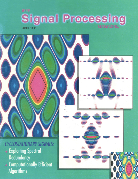
The most widely cited single article introducing the subject of cyclostationarity is entitled “Exploitation of Spectral Redundancy in Cyclostationary Signals” and, as of this writing (2018), was published almost three decades ago (1991) in the IEEE Signal Processing Society’s IEEE Signal Processing Magazine vol. 8 (2), pp. 14-36. According to Google Scholar as of 1 July 2018, this tutorial article has been cited in 1,217 research papers and, as of this update on 19 October 2021,1404 papers. This represents a current 3-year-average growth rate of almost five new citations every month in its 30th year. Based on this evidence, it appears that this introductory article on cyclostationarity has been the most popular among researchers, and visitors to this website are therefore referred to this article for the first recommended reading. The link [JP36] provides free access to the entire special issue.
Fifteen years later, in 2006, the most comprehensive survey of cyclostationarity at that time, entitled “Cyclostationarity: Half a Century of Research”, was published in the European Association for Signal Processing Journal Signal Processing vol. 86 (4), pp. 639-697. According to Google Scholar as of 1 July 2018, this survey had been cited in 740 research papers and, as of this update on 19 October 2021,1042 papers. This represents a current 3-year-average growth rate of almost eight new citations every month in its 15th year. This survey paper received from the Publisher (Elsevier) the “Most Cited Paper Award” in 2008; and, each year since its first appearance online up through 2011, it was the most cited paper among those published in Signal Processing in the previous five years, and among the top 10 most downloaded papers from Signal Processing. Based on this evidence, it appears that this comprehensive survey paper on cyclostationarity has been the most popular among researchers, and visitors to this website are therefore referred to this paper [JP64] for the second recommended reading. However, for new students of this subject, it is recommended that this survey paper not be read thoroughly at this stage; it should just be perused to widen one’s perspective on the scope of this subject as of 2006.
For visitors to this website looking for an introduction to the 2nd order (or wide-sense) theory of cyclostationarity at an intermediate level—more technical than the magazine article cited above but less technical and considerably less comprehensive than the survey paper also cited above—the journal paper entitled “The Spectral Correlation Theory of Cyclostationary Time-Series” [JP15] is recommended. This paper was published in 1986 in the Journal Signal Processing, Vol. 11, pp. 13-36. An indication that this paper was well received is the fact that it was awarded the best paper of the year by the European Association for Signal Processing. In contrast to the 1,217 citations of the magazine article recommended above, this journal paper had been cited in only 351 research papers as of 1 July 2018 but, as of this update on 19 October 2021, its citations have grown to 431, a 3-year rate of two new citations every month in its 35th year. It is suggested here that this lesser popularity more reflects differences in the readerships of the 1991 magazine and this 1986 journal than it reflects the utility of the paper.
The textbooks/reference-books about cyclostationarity that have been the most frequently cited in research papers as of this writing (2018) and again, as of this update on 19 October 2021, are the following three books which, together, comprise over 1600 pages and have been cited in 3,080 research papers over the last three decades.
One more recommendation for students of cyclostationarity is Chapter 1 in the above cited book [Bk5], which provides an introduction to the subject that is considerably broader and deeper than the introductions in the articles [JP15] and [JP36], also cited above. In fact, in the ensuing 25 years since publication of [Bk5], no other introductions even approaching the breadth and depth of this chapter can be found in the literature.
The above seven recommended readings have been cited in nearly 6000 research papers tracked by Google Scholar. This averages 200 citations per year for 30 years. For emphasis, at the cost of being redundant, it is stated here before moving on that these citation statistics provide the basis for the WCM’s selection, from among all published tutorial treatments of cyclostationarity, of this particular set of seven. It will not go unnoticed that everyone of these recommended readings was written by the WCM. No other treatments that are as popular as these are known to the WCM.
However, as of late 2019, there has been a major step forward in the publication of comprehensive book treatments of cyclostationarity that can be highly recommended for serious students of the subject: Cyclostationary Processes and Time Series: Theory, Applications, and Generalizations, by Professor Antonio Napolitano, the most prolific contributor to this field for two decades now. Besides providing the most comprehensive treatment of the subject—a treatment that is both mathematical and very readable—including both the FOT probability theory and the stochastic probability theory of almost cyclostationary time series or processes and all established generalizations of these (discussed in the following section of this page), this book also is the most scholarly treatment since the seminal book [Bk2]. Being a historian of time-series analysis, I can say with confidence that no other treatment of the history of contributions to the theory of cyclostationarity can compete with this exemplary book. It will be *the* definitive treatment covering the period from the inception of this subject of study to the end of 2019 (more than half a century) for the foreseeable future.
Higher-Order Cyclostationarity
Although the first comprehensive treatment of cyclostationarity focused on the theory of 2nd-order temporal and spectral moments and appeared in 1987 [Bk2], a similarly comprehensive theory of higher-order temporal and spectral moments did not appear for another 7 years: [JP55], [JP56], four years after the first introduction of nth-order spectral moments for cyclostationary time series [B2, Ref. Gardner 1990c]. This theory, which is based on Fraction-of-Time Probability exposed a number of issues with the alternative theory of higher-order moments based on stochastic processes—both stationary and cyclostationary. It also led to the discovery of an entirely new interpretation of cumulants, one which makes no reference to the more abstract stochastic process. Rather, the cumulant is derived as the answer to the question “how does one calculate the strength and phase of a pure-nth-order sine wave from a time series exhibiting cyclostationarity?” The question does not involve classical probability or stochastic processes; yet its answer is “calculate the nth-order cyclic cumulant” which is a function of the cyclic moments in the FOT-Probability Theory. The 2-part paper [JP55], [JP56] is the WCM’s first recommended reading on this subject of higher-order cyclostationarity. The second recommendation is Section 13 of the comprehensive survey paper [JP64], and the third recommendation is Chapter 4 in the encyclopedic book [B2], both of which contain references to diverse sources. Other recommended reading is the book chapter [BkC3] and chap. 2 in the book [Bk5]. According to Google Scholar as of April 2022, the number of citations of [JP55] and [JP56] is 352 and 261, respectively. In comparison with the citations numbers given above on this Page 2, this subject appears to be only about 1/3 as popular as the second-order theory. This likely reflects the smaller number of practical applications of the higher-order theory. Yet, there are some interesting applications where the higher-order theory is essential (see [JP64] and Sec. 4.9 in [B2]).
Relative to the aforementioned three introductory but thorough treatments of cyclostationarity, there is one textbook/reference-book that is highly complementary and can be strongly recommended for advanced study, entitled Generalizations of Cyclostationary Signal Processing: Spectral Analysis and Applications. The generalizations of cyclostationarity introduced in this unique book are summarized on Page 5.
An even more recent development of the cyclostationarity paradigm is its extension to signals that exhibit irregular cyclicity, rather than the regular cyclicity we call cyclostationarity. This extension enables application of cyclostationarity theory and method to time-series data originating in many fields of science where there are cyclic influences on data (observations and measurements on natural systems), but for which the cyclicity is irregular as it typically is in nature. This extension originates in the work presented in the article “Statistically Inferred Time Warping: Extending the Cyclostationarity Paradigm from Regular to Irregular Statistical Cyclicity in Scientific Data,” written in 2016 and published in 2018 [JP65]; see also [J39].
However, from an educational perspective, visitors to this website whose objective is to develop a firm command of not only the mathematical principles and models of cyclostationarity but also the conceptual link between the mathematics and empirical data—a critically important link that enables the user to insightfully design or even just correctly use algorithms for signal processing (time-series data analysis)—are strongly urged to take a temporary detour away from cyclostationarity per se and toward the fundamental question:
“What should be the role of the theory of probability and stochastic processes in the conceptualization of cyclostationarity and even stationarity?”
As discussed in considerable detail on Page 3, one can argue quite convincingly that, from a scientific and engineering perspective, a wrong step was taken back around the middle of the 20th Century in the nascent field of time-series analysis (more frequently referred to as signal processing today) when the temporal counterpart referred to here—introduced by Norbert Wiener in his 1949 book, Extrapolation, Interpolation, and Smoothing of Stationary Time Series, with Engineering Applications—was rejected by mathematicians in favor of Ensemble Statistics, Probability, and Stochastic Processes. This step away from the more concrete conceptualization of statistical signal processing that was emerging and toward a more abstract mathematical model, called a stochastic process, is now so ingrained in what university students are taught today, that few STEM (Science, Technology, Engineering, and Mathematics) professors and practitioners are even aware of the alternative that is, on this website, argued to be superior for the great majority of real-world applications—the only advantage of stochastic processes being their amenability to mathematical proof-making, despite the fact that it is typically impossible to verify that real-world data satisfies the axiomatic assumptions upon which the stochastic process model is based! In essence, the assumptions pave the way for constructing mathematical proofs in the theory of stochastic processes, not—as they should in science—pave the way for validating applicability of theory to real-world applications.
This is an extremely serious mis-step for this important field of study and it parallels a similar egregious mis-step taken early on in the 20th Century when astrophysics and cosmology became dominated by mathematicians who were bent on developing a theory that was particularly mathematically viable, rather than being most consistent with the Scientific Method. This led to wildly abstract models and associated theory (such as black holes, dark matter, dark energy, and the like) that are dominated by the role of the force of Gravity, whereas Electromagnetism has been scientifically demonstrated to play the true central role in the workings of the Universe. As in the case of the firmly established but mistaken belief that stochastic process models for stationary and cyclostationary time-series are the only viable models, the gravity-centric model of the universe, upon which all mainstream astrophysics is based, is so ingrained in what university students have been taught since early in the 20th century, that few professors and mainstream astrophysics practitioners can bring themselves to recognize the alternative electromagnetism-centric model that is strongly argued to be superior in terms of agreeing with empirical data. Interested readers are referred to the major website www.thunderbolts.info, where the page “Beginner’s Guide” is a good place to start.
With this hindsight, this website would be remiss to simply present the subject of cyclostationarity within the framework of stochastic processes, which has unfortunately become the norm. This would be the path of least resistance considering the impact of over half a century of using and teaching the stochastic process theory as if it was the only viable theory, not even mentioning the fact that an alternative exists and actually preceded the stochastic process concept before it was buried by mathematicians behaving as if the scientific method was irrelevant.
FOREWORD
A good deal of our statistical theory, although it is mathematical in nature, originated not in mathematics but in problems of astronomy, geomagnetism and meteorology: examples of fruitful problems in these subjects have included the clustering of stars, also galaxies, on the celestial sphere, tidal analysis, the correlation of fluctuations of the Earth’s magnetic field with other solar-terrestrial effects, and the determination of seasonal variations and climatic trends from weather data. All three of these fields are observational. Great figures of the past, such as C. F. Gauss (1777—1855) (who worked with both astronomical and geomagnetic data, and discovered the method of least square fitting of data, the normal error distribution, and the Fast Fourier Transform algorithm), have worked on observational data analysis and have contributed much to our body of knowledge on time series and randomness.
Much other theory has come from gambling, gunnery, and agricultural research, fields that are experimental. Measurements of the fall of shot on a firing range will reveal a pattern that can be regarded as a sample from a normal distribution in two dimensions, together with whatever bias is imposed by pointing and aiming, the wind, air temperature, atmospheric pressure and Earth rotation. The deterministic part of any one of these influences may be characterized with further precision by further firing tests. In the experimental sciences, as well as in the observational, great names associated with the foundations of statistics and probability also come to mind.
Experimental subjects are traditionally distinguished from observational ones by the property that conditions are under the control of the experimenter. The design of experiments leads the experimenter to the idea of an ensemble, or random process, an abstract probabilistic creation illustrated by the bottomless barrel of well-mixed marbles that is introduced in elementary probability courses. A characteristic feature of the contents of such a barrel is that we know in advance how many marbles there are of each color, because it is we who put them in; thus, a sample set that is withdrawn after stirring must be compatible with the known mix.
The observational situation is quite unlike this. Our knowledge of what is in the barrel, or of what Nature has in store for us, is to be deduced from what has been observed to come out of the barrel, to date. The probability distribution, rather than being a given, is in fact to be intuited from experience. The vital stage of connecting the world of experience to the different world of conventional probability theory may be glossed over when foreknowledge of the barrel and its contents — a probabilistic model — are posited as a point of departure. Many experimental situations are like this observational one.
The theory of signal processing, as it has developed in electrical and electronics engineering, leans heavily toward the random process, defined in terms of probability distributions applicable to ensembles of sample signal waveforms. But many students who are adept at the useful mathematical techniques of the probabilistic approach and quite at home with joint probability distributions are unable to make even a rough drawing of the underlying sample waveforms. The idea that the sample waveforms are the deterministic quantities being modeled somehow seems to get lost.
When we examine the pattern of fall of shot from a gun, or the pattern of bullet holes in a target made by firing from a rifle clamped in a vise, the distribution can be characterized by its measurable centroid and second moments or other spread parameters. While such a pattern is necessarily discrete, and never much like a normal distribution, we have been taught to picture the pattern as a sample from an infinite ensemble of such patterns; from this point of view the pattern will of course be compatible with the adopted parent population, as with the marbles. In this probabilistic approach, to simplify mathematical discussion, one begins with a model, or specification of the continuous probability distribution from which each sample is supposed to be drawn. Although this probability distribution is not known, one is comforted by the assurance that it is potentially approachable by expenditure of more ammunition. But in fact it is not.
The assumption of randomness is an expression of ignorance. Progress means the identification of systematic effects which, taken as a whole, may initially give the appearance of randomness or unpredictability. Continuing to fire at the target on a rifle range will not refine the probability distribution currently in use but will reveal, to a sufficiently astute planner of experiments, that air temperature, for example, has a determinate effect which was always present but was previously accepted as stochastic. After measurement, to appropriate precision, temperature may be allowed for. Then a new probability model may be constructed to cover the effects that remain unpredictable.
Many authors have been troubled by the standard information theory approach via the random process or probability distribution because it seems to put the cart before the horse. Some sample parameters such as mean amplitudes or powers, mean durations and variances may be known, to precision of measurement, but if we are to go beyond pure mathematical deduction and make advances in the realm of phenomena, theory should start from the data. To do otherwise risks failure to discover that which is not built into the model. Estimating the magnitude of an earthquake from seismograms, assessing a stress-test cardiogram, or the pollutant in a stormwater drain, are typical exercises where noise, systematic or random, is to be fought against. Problems on the forefront of development are often ones where the probability distributions of neither signal nor noise is known; and such distributions may be essentially unknowable because repetition is impossible. Thus, any account of measurement, data processing, and interpretation of data that is restricted to probabilistic models leaves something to be desired.
The techniques used in actual research with real data do not loom large in courses in probability. Professor Gardner’s book demonstrates a consistent approach from data, those things which in fact are given, and shows that analysis need not proceed from assumed probability distributions or random processes. This is a healthy approach and one that can be recommended to any reader.
Ronald N. Bracewell
Stanford, California
PREFACE
This book grew out of an enlightening discovery I made a few years ago, as a result of a long-term attempt to strengthen the tenuous conceptual link between the abstract probabilistic theory of cyclostationary stochastic processes and empirical methods of signal processing that accommodate or exploit periodicity in random data. After a period of unsatisfactory progress toward using the concept of ergodicity1 to strengthen this link, it occurred to me (perhaps wishfully) that the abstraction of the probabilistic framework of the theory might not be necessary. As a first step in pursuing this idea, I set out to clarify for myself the extent to which the probabilistic framework is needed to explain various well-known concepts and methods in the theory of stationary stochastic processes, especially spectral analysis theory. To my surprise, I discovered that all the concepts and methods of empirical spectral analysis can be explained in a more straightforward fashion in terms of a deterministic theory, that is, a theory based on time-averages of a single time-series rather than ensemble-averages of hypothetical random samples from an abstract probabilistic model. To be more specific, I found that the fundamental concepts and methods of empirical spectral analysis can be explained without use of probability calculus or the concept of probability and that probability calculus, which is indeed useful for quantification of the notion of degree of randomness or variability, can be based on time-averages of a single time-series without any use of the concept or theory of a stochastic process defined on an abstract probability space. This seemed to be of such fundamental importance for practicing engineers and scientists and so intuitively satisfying that I felt it must already be in the literature.
To put my discovery in perspective, I became a student of the history of the subject. I found that the apparent present-day complacence with the abstraction of the probabilistic theory of stochastic processes, introduced by A. N. Kolmogorov in 1941, has been the trend for about 40 years (as of 1985). Nevertheless, I found also that many probabilists throughout this period, including Kolmogorov himself, have felt that the concept of randomness should be defined as directly as possible, and that from this standpoint it seems artificial to conceive of a time-series as a sample of a stochastic process. (The first notable attempt to set up the probability calculus more directly was the theory of Collectives introduced by Von Mises in 1919; the mathematical development of such alternative approaches is traced by P. R. Masani [Masani 1979].) In the engineering literature, I found that in the early 1960s two writers, D. G. Brennan [Brennan 1961] and E. M. Hofstetter [Hofstetter 1964], had made notable efforts to explain that much of the theory of stationary time-series need not be based on the abstract probabilistic theory of stochastic processes and then linked with empirical method only through the abstract concept of ergodicity, but rather that a probabilistic theory based directly on time-averages will suffice; however, they did not pursue the idea that a theory of empirical spectral analysis can be developed without any use of probability. Similarly, the more recent book by D. R. Brillinger on time-series [Brillinger 1975] briefly explains precisely how the probabilistic theory of stationary time-series can be based on time-averages, but it develops the theory of empirical spectral analysis entirely within the probabilistic framework. Likewise, the early engineering book by R. B. Blackman and J. W. Tukey [Blackman and Tukey 1958] on spectral analysis defines an idealized spectrum in terms of time-averages but then carries out all analysis of measurement techniques within the probabilistic framework of stochastic processes. In the face of this 40-year trend, I was perplexed to find that the one most profound and influential work in the entire history of the subject of empirical spectral analysis, Norbert Wiener’s Generalized Harmonic Analysis, written in 1930 [Wiener 1930], was entirely devoid of probability theory; and yet I found only one book written since then for engineers or scientists that provides more than a brief mention of Wiener’s deterministic theory. All other such books that I found emphasize the probabilistic theory of A. N. Kolmogorov usually to the complete exclusion of Wiener’s deterministic theory. This one book was written by a close friend and colleague of Wiener’s, Y. W. Lee, in 1960 [Lee 1960]. Some explanation of this apparent historical anomaly is given by P. R. Masani in his recent commentary on Wiener’s Generalized Harmonic Analysis [Masani 1979]: “The quick appearance of the Birkhoff ergodic theorem and the Kolmogorov theory of stochastic processes after the publication of Wiener’s Generalized Harmonic Analysis created an intellectual climate favoring stochastic analysis rather than generalized harmonic analysis.” But Masani goes on to explain that the current opinion, that Wiener’s 1930 memoir [Wiener 1930] marks the culmination of generalized harmonic analysis and its supersession by the more advanced theories of stochastic processes, is questionable on several counts, and he states that the “integrity and wisdom” in the attitude expressed in the early 1960s by Kolmogorov suggesting a possible return to the ideas of Von Mises “. . . should point the way toward the future. Side by side with the vigorous pursuit of the theory of stochastic processes, must coexist a more direct process-free [deterministic] inquiry of randomness of different classes of functions.”
As a result of my discovery and my newly gained historical perspective, I felt compelled to write a book that would have the same goals, in principle, as many existing books on spectral analysis—to present a general theory and methodology for empirical spectral analysis—but that would present a more relevant and palatable (for many applications) deterministic theory following Wiener’s original approach rather than the conventional probabilistic theory. As the book developed, I continued to wonder about the apparent fact that no one in the 50 years (as of 1985) since Wiener’s memoir had considered such a project worthy enough to pursue. However, as I continued to search the literature, I found that one writer, J. Kampé de Fériet. did make some progress along these lines in a tutorial paper [Kampé de Fériet 1954], and other authors have contributed to development of deterministic theories of related subjects in time-series analysis, such as linear prediction and extrapolation [Wold 1948], [Finch 1969], [Fine 1970]. Furthermore, as the book progressed and I observed the favorable reactions of my students and colleagues, my conviction grew to the point that I am now convinced that it is generally beneficial for students of the subject of empirical spectral analysis to study the deterministic theory before studying the more abstract probabilistic theory.
When I had completed most of the development for a book on a deterministic theory of empirical spectral analysis of stationary time-series, I was then able to return to the original project of presenting the results of my research work on cyclostationary time-series but within a nonprobabilistic framework. Once I started, it quickly became apparent that I was able to conceptualize intuitions, hunches, conjectures, and so forth far more clearly than before when I was laboring within the probabilistic framework. The original relatively fragmented research results on cyclostationary stochastic processes rapidly grew into a comprehensive theory of random time-series from periodic phenomena that is every bit as satisfying as the theory of random time-series from constant phenomena (stationary time-series) and is even richer. This theory, which brings to light the fundamental role played by spectral correlation in the study of periodic phenomena, is presented in Part II.
Part I of this book is intended to serve as both a graduate-level textbook and a technical reference. The only prerequisite is an introductory course on Fourier analysis. However, some prior exposure to probability would be helpful for Section B in Chapter 5 and Section A in Chapter 15. The body of the text in Part I presents a thorough development of fundamental concepts and results in the theory of statistical spectral analysis of empirical time-series from constant phenomena, and a brief overview is given at the end of Chapter 1. Various supplements that expand on topics that are in themselves important or at least illustrative but that are not essential to the foundation and framework of the theory, are included in appendices and exercises at the ends of chapters.
Part II of this book, like Part I, is intended to serve as both textbook and reference, and the same unifying philosophical framework developed in Part I is used in Part II. However, unlike Part I, the majority of concepts and results presented in Part II are new. Because of the novelty of this material, a brief preview is given in the Introduction to Part II. The only prerequisite for Part II is Part I.
The focus in this book is on fundamental concepts, analytical techniques. and basic empirical methods. In order to maintain a smooth flow of thought in the development and presentation of concepts that steadily build on one another, various derivations and proofs are omitted from the text proper, and are put into the exercises, which include detailed hints and outlines of solution approaches. Depending on students’ background, instructors can either assign these as homework exercises, or present them in the lectures. Because the treatment of experimental design and applications is brief and is also relegated to the exercises and concise appendices, some readers might desire supplements on these topics.
===============
1 Ergodicity is the property of a mathematical model for an infinite set of time-series that guarantees that an ensemble average over the infinite set will equal an infinite time average over one member of the set.
REFERENCES
BLACKMAN, R. B. and J, W. TUKEY. 1958. The Measurement of Power Spectra. New York: American Telephone and Telegraph Co.
BRENNAN, D. G. 1961. Probability theory in communication system engineering, Chapter 2 in Communication System Theory. Ed. E. J. Baghdady, New York: McGraw-Hill.
BRILLINGER, D. R. 1975. Time Series. New York: Holt, Rinehart and Winston.
FINCH, P. D. 1969. Linear least squares prediction in non-stochastic time-series. Advances in Applied Prob. 1:111—22.
FINE, T. L. 1970. Extrapolation when very little is known about the source. Information and Control. 16:33 1—359.
HOFSTETTER, E. M. 1964. Random processes. Chapter 3 in The Mathematics of Physics and Chemistry, vol. 11. Ed. H. Margenau and G. M. Murphy. Princeton, N.J.: D. Van Nostrand Co.
KAMPÉ DE FÉRIET, J. 1954. Introduction to the statistical theory of turbulence. I and 11. J. Soc. Indust. Appl. Math. 2, Nos. I and 3:1—9 and 143—174.
LEE, Y. W. 1960. Statistical Theory of Communication. New York: John Wiley & Sons.
MASANI, P. R. 1979. “Commentary on the memoir on generalized harmonic analysis.” pp. 333—379 in Norbert Wiener: Collected Works, Volume II. Cambridge. Mass.: Massachusetts Institute of Technology.
WIENER, N. 1930. Generalized harmonic analysis. Acta Mathematika. 55:117—258.
WOLD, H. O. A. 1948. On prediction in stationary time-series. Annals of Math Stat. 19:558—567.
William A. Gardner
INTRODUCTION
The subject of Part I is the statistical spectral analysis of empirical time-series. The term empirical indicates that the time-series represents data from a physical phenomenon; the term spectral analysis denotes decomposition of the time-series into sine wave components; and the term statistical indicates that the squared magnitude of each measured or computed sine wave component, or the product of pairs of such components, is averaged to reduce random effects in the data that mask the spectral characteristics of the phenomenon under study. The purpose of Part I is to present a comprehensive deterministic theory of statistical spectral analysis and thereby to show that contrary to popular belief, the theoretical foundations of this subject need not be based on probabilistic concepts. The motivation for Part I is that for many applications the conceptual gap between practice and the deterministic theory presented herein is narrower and thus easier to bridge than is the conceptual gap between practice and the more abstract probabilistic theory. Nevertheless, probabilistic concepts are not ignored. A means for obtaining probabilistic interpretations of the deterministic theory is developed in terms of fraction-of-time distributions, and ensemble averages are occasionally discussed.
A few words about the terminology used are in order. Although the terms statistical and probabilistic are used by many as if they were synonymous, their meanings are quite distinct. According to the Oxford English Dictionary, statistical means nothing more than “consisting of or founded on collections of numerical facts”. Therefore, an average of a collection of spectra is a statistical spectrum. And this has nothing to do with probability. Thus, there is nothing contradictory in the notion of a deterministic or non-probabilistic theory of statistical spectral analysis. (An interesting discussion of variations in usage of the term statistical is given in Comparative Statistical Inference by V. Barnett [Barnett 1973]). The term deterministic is used here as it is commonly used, as a synonym for non-probabilistic. Nevertheless, the reader should be forewarned that the elements of the non-probabilistic theory presented herein are defined by infinite limits of time averages and are therefore no more deterministic in practice than are the elements of the probabilistic theory. (In mathematics, the deterministic and probabilistic theories referred to herein are sometimes called the functional and stochastic theories, respectively.) The term random is often taken as an implication of an underlying probabilistic model. But in this book, the term is used in its broader sense to denote nothing more than the vague notion of erratic unpredictable behavior.
This introductory chapter sets the stage for the in-depth study of spectral analysis taken up in the following chapters by explaining objectives and motives, answering some basic questions about the nature and uses of spectral analysis, and establishing a historical perspective on the subject.
A premise of this book is that the way engineers and scientists are commonly taught to think about empirical statistical spectral analysis of time-series data is fundamentally inappropriate for many applications—maybe even most. The essence of the subject is not really as abstruse as it appears to be from what has become the conventional point of view. The problem is that the subject has been imbedded in the abstract probabilistic framework of stochastic processes, and this abstraction impedes conceptualization of the fundamental principles of empirical statistical spectral analysis. To circumvent this artificial conceptual complication, the probabilistic theory of statistical spectral analysis should be taught to engineers and scientists only after they have learned the fundamental deterministic principles—both qualitative and quantitative. For example, one should first learn 1) when and why sine wave analysis of time-series is appropriate, 2) how and why temporal and spectral resolution interact, 3) why statistical (averaged) spectra are of interest, and 4) what the various methods for measuring and computing statistical spectra are and how they are related. One should also learn 5) how simultaneously to control the spectral and temporal resolution and the degree of randomness (reliability) of a statistical spectrum. All this can be accomplished in a non-superficial way without reference to the probabilistic theory of stochastic processes.
The concept of a deterministic theory of statistical spectral analysis is not new. Much deterministic theory was developed prior to and after the infusion, beginning in the 1930s, of probabilistic concepts into the field of time-series analysis. The most fundamental concept underlying present-day theory of statistical spectral analysis is the concept of an ideal spectrum, and the primary objective of statistical spectral analysis is to estimate the ideal spectrum using a finite amount of data. The first theory to introduce the concept of an ideal spectrum is Norbert Wiener’s theory of generalized harmonic analysis [Wiener 1930], and this theory is deterministic. Later, Joseph Kampé de Fériet presented a deterministic theory of statistical spectral analysis that ties Wiener’s theory more closely to the empirical reality of finite-length time-series [Kampé de Fériet 1954]. But the very great majority of treatments in the ensuing 30 years consider only probabilistic theory of statistical spectral analysis that is based on the use of stochastic process models of time functions, although a few authors do briefly mention the dual deterministic theory (e.g., [Koopmans 1974; Brillinger 1976]).
The primary objective of Part I of this book is to adopt the deterministic viewpoint of Wiener and Kampé de Fériet and show that a comprehensive deterministic theory of statistical spectral analysis, which for many applications relates more directly to empirical reality than does its more popular probabilistic counterpart based on stochastic processes, can be developed. A secondary objective of Part I is to adopt the empirical viewpoint of Donald G. Brennan [Brennan 1961] and Edward M. Hofstetter [Hofstetter 1964], from which they develop an objective probabilistic theory of stationary random processes based on fraction-of-time distributions, and show that probability theory can be applied to the deterministic theory of statistical spectral analysis without introducing the more abstract mathematical model of empirical reality based on the axiomatic or subjective probabilistic theory of stochastic processes. This can be interpreted as an exploitation of Herman O. A. Wold’s isomorphism between an empirical time-series and a probabilistic model of a stationary stochastic process. As explained below in Section B, this isomorphism is constructed by defining the ensemble, upon which the probabilistic theory of time functions is based, to be the set of all time-translated versions of a single function of time—the ensemble generator—and it is responsible for the duality between probabilistic (ensemble-average) and deterministic (time-average) theories of time-series [Wold 1948] [Gardner 1985]. Moreover, the excuse generally offered for adopting a stochastic process model when it is admitted that it is time averages, not ensemble averages, that are of interest in practice is to carelessly assume that the stochastic process is ergodic (an even more abstract concept), in which case time-averages converge to ensemble averages—a result typically presented to students as magic; what is not generally mentioned (and probably rarely even recognized by instructors) is that assuming ergodicity is tantamount to assuming the ensemble is (with probability equal to one) simply the collection of all time-translated versions of a single time function. Thus, the whole exercise of abandoning the more straightforward fraction-of-time probabilistic model in favor of the abstract stochastic process model is all for naught. So why drag our students through this silly exercise that is bound to serve no purpose other than to confuse them, especially given that the truth about all this presented here is essentially never revealed to the student.
There are two motives for Part I of this book. The first is to stimulate a reassessment of the way engineers and scientists are today, evidently exclusively, taught to think about statistical spectral analysis by showing that probability theory need not play a primary role. The second motive is to pave the way for introducing a new theory and methodology for statistical spectral analysis of random data from periodically time-variant phenomena, which is presented in Part II. The fact that this new theory and methodology, which unifies various emerging—as well as long-established—time-series analysis concepts and techniques, is most transparent when built on the foundation of the deterministic theory developed in Part I is additional testimony that probability theory need not play a primary role in statistical spectral analysis.
The book, although concise, is tutorial and is intended to be comprehensible by graduate students and professionals in engineering, science, mathematics, and statistics. The accomplishments of the book should be appreciated most by those who have studied statistical spectral analysis in terms of the popular probabilistic theory and have struggled to bridge the conceptual gaps between this abstract theory and empirical reality.
Spectral analysis of functions is used for solving a wide variety of practical problems encountered by engineers and scientists in nearly every field of engineering and science. The functions of primary interest in most fields involving data analysis are temporal or spatial waveforms or discrete sequences of numbers. The most basic purpose of spectral analysis is to represent a function by a sum of weighted sinusoidal functions called spectral components; that is, the purpose is to decompose (analyze) a function into these spectral components. The weighting function in the decomposition is a density of spectral components. This spectral density is also called a spectrum1. The reason for representing a function by its spectrum is that the spectrum can be an efficient, convenient, and often revealing description of the function.
As an example of the use of spectral representation of temporal waveforms in the field of signal processing, consider the signal extraction problem of extracting an information-bearing signal from corrupted (noisy) measurements. In many situations, the spectrum of the signal differs substantially from the spectrum of the noise. For example, the noise might have more high-frequency content; hence, the technique of spectral filtering can be used to attenuate the noise while leaving the signal intact. Another example is the data-compression problem of using coding to compress the amount of data used to represent information for the purpose of efficient storage or transmission. In many situations, the information contained in a complex temporal waveform (e.g., a speech segment) can be coded more efficiently in terms of the spectrum.
There are two types of spectral representations. The more elementary of the two shall be referred to as simply the spectrum, and the other shall be referred to as the statistical spectrum. The term statistical indicates that averaging or smoothing is used to reduce random effects in the data that mask the spectral characteristics of the phenomenon under study. For time-functions, the spectrum is obtained from an invertible transformation from a time-domain description of a function,  , to a frequency-domain description, or more generally to a joint time- and frequency-domain description. The (complex) spectrum of a segment of data of length
  centered at time
  and evaluated at frequency
  is
is
(1) ![\[ X_{T}(t, f) \triangleq \int_{t-T / 2}^{t+T / 2} x(u) e^{-i 2 \pi f u} d u, \]](https://cyclostationarity.com/wp-content/ql-cache/quicklatex.com-61d97d6f201d6c0a9176cb6e8bbe9ce3_l3.svg "Rendered by QuickLaTeX.com")
for which  . Because of the invertibility of this transformation, a function can be recovered from its spectrum,
(2) ![\[ x(u)=\int_{-\infty}^{\infty} X_{T}(t, f) e^{i 2 \pi f u} d f, \quad u \in[t-T / 2, t+T / 2]. \]](https://cyclostationarity.com/wp-content/ql-cache/quicklatex.com-2b1aaa144687c78582683a9a1c6c70a4_l3.svg "Rendered by QuickLaTeX.com")
In contrast to this, a statistical spectrum involves a magnitude-extraction operation that is not invertible followed by an averaging or smoothing operation. For example, the statistical spectrum
(3) ![\[ S_{x_{T}}(t, f)_{\Delta t} \triangleq \frac{1}{\Delta t} \int_{t-\Delta t / 2}^{t+\Delta t / 2} S_{x_{T}}(v, f) d v, \]](https://cyclostationarity.com/wp-content/ql-cache/quicklatex.com-f7bedb901c9416a2b839f8fb5fe528a0_l3.svg "Rendered by QuickLaTeX.com")
is obtained from the normalized squared magnitude spectrum
(4) ![\[ S_{x_{T}}(t, f) \triangleq \frac{1}{T}\left|X_{T}(t, f)\right|^{2} , \]](https://cyclostationarity.com/wp-content/ql-cache/quicklatex.com-f9889fbb83b1a600e1a41b20fe653200_l3.svg "Rendered by QuickLaTeX.com")
followed by a temporal smoothing operation. Thus, a statistical spectrum is a summary description of a function from which the function cannot be recovered. Therefore, although the spectrum is useful for both signal extraction and data compression, the statistical spectrum is not directly useful for either. It is, however, quite useful indirectly for analysis, design, and adaptation of schemes for signal extraction and data compression. It is also useful for forecasting or prediction and more directly for other signal-processing tasks such as 1) the modeling and system-identification problems of determining the characteristics of a system from measurements on it, such as its response to excitation, and 2) decision problems, such as the signal-detection problem of detecting the presence of a signal buried in noise. As a matter of fact, the problem of detecting hidden periodicities in random data motivated the earliest work in the development of spectral analysis, as discussed in Section D below.
Statistical spectral analysis has diverse applications in areas such as mechanical vibrations, acoustics, speech, communications, radar, sonar, ultrasonics, optics, astronomy, meteorology, oceanography, geophysics, economics, biomedicine, and many other areas. To be more specific, let us briefly consider a few applications. Spectral analysis is used to characterize various signal sources. For example, the spectral purity of a sine wave source (oscillator) is determined by measuring the amounts of harmonics from distortion due, for example, to nonlinear effects in the oscillator and also by measuring the spectral content close in to the fundamental frequency of the oscillator, which is due to random phase noise. Also, the study of modulation and coding of sine wave carrier signals and pulse-train signals for communications, telemetry, radar, and sonar employs spectral analysis as a fundamental tool, as do surveillance systems that must detect and identify modulated and coded signals in a noisy environment. Spectral analysis of the response of electrical networks and components such as amplifiers to both sine wave and random-noise excitation is used to measure various properties such as nonlinear distortion, rejection of unwanted components, such as power-supply components and common-mode components at the inputs of differential amplifiers, and the characteristics of filters, such as center frequencies, bandwidths, pass-band ripple, and stop-band rejection. Similarly, spectral analysis is used to study the magnitude and phase characteristics of the transfer functions as well as nonlinear distortion of various electrical, mechanical, and other systems, including loudspeakers, communication channels and modems (modulator-demodulators), and magnetic tape recorders in which variations in tape motion introduce signal distortions. In the monitoring and diagnosis of rotating machinery, spectral analysis is used to characterize random vibration patterns that result from wear and damage that cause imbalances. Also, structural analysis of physical systems such as aircraft and other vehicles employs spectral analysis of vibrational response to random excitation to identify natural modes of vibration (resonances). In the study of natural phenomena such as weather and the behavior of wildlife and fisheries populations, the problem of identifying cause-effect relationships is attacked using techniques of spectral analysis. Various physical theories are developed with the assistance of spectral analysis, for example, in studies of atmospheric turbulence and undersea acoustical propagation. In various fields of endeavor involving large, complex systems such as economics, spectral analysis is used in fitting models to time-series for several purposes, such as simulation and forecasting. As might be surmised from this sampling of applications, the techniques of spectral analysis permeate nearly every field of science and of engineering.
Spectral analysis applies to both continuous-time functions, called waveforms, and discrete-time functions, called sampled data. Other terms are commonly used also; for example, the terms data and time-series are each used for both continuous-time and discrete-time functions. Since the great majority of data sources are continuous-time phenomena, continuous-time data are focused on in this book, because an important objective is to maintain a close tie between theory and empirical reality. Furthermore, since optical technology has emerged as a new frontier in signal processing and optical quantities vary continuously in time and space, this focus on continuous time data is well suited to upcoming technological developments. Nevertheless, since some of the most economical implementations of spectrum analyzers and many of the newly emerging parametric methods of spectral analysis operate with discrete time and discrete frequency and since some data are available only in discrete form, discrete-time and discrete-frequency methods also are described.
===============
1 The term spectrum, which derives from the Latin for image, was originally introduced by Sir Isaac Newton (see [Robinson 1982]).
The primary reason why sinewaves are especially appropriate components with which to analyze waveforms is our preoccupation with convolutions of time series with the kernels (impulse-response functions) of linear time-invariant (LTI) transformations, which we often call filters. A secondary reason why statistical (time-averaged) analysis into sinewave components is especially appropriate is our preoccupation with time-invariant phenomena (data sources). To be specific, a transformation of a waveform into another waveform, say  , is an LTI transformation if and only if there exists a weighting function
  (here assumed to be absolutely integrable in the generalized sense, which accommodates Dirac deltas) such that is the convolution (denoted by
  ) of with :
(5) ![\[ \begin{aligned} y(t) = x(t) \otimes h(t) &=\int_{-\infty}^{\infty} h(t-u) x(u) d u \\ &=\int_{-\infty}^{\infty} h(v) x(t-v) d v \end{aligned} \]](https://cyclostationarity.com/wp-content/ql-cache/quicklatex.com-112f5cfa232c1dd87430d18ee3b299d3_l3.svg "Rendered by QuickLaTeX.com")
The time-invariance property of a transformation is, more precisely, a translation- invariance property that guarantees that a translation, by  , of to
  has no effect on other than a corresponding translation to
  (exercise 1). A phenomenon is said to be time-invariant only if it is persistent in the sense that it is appropriate to conceive of a mathematical model of for which the following limit time-average exists for each value of
  and is not identically zero,3
(6) ![\[ \hat{R}_{x}(\tau) \triangleq \lim _{T \rightarrow \infty} \frac{1}{T} \int_{-T/ 2}^{T / 2} x\left(t+\frac{\tau}{2}\right)x\left(t-\frac{\tau}{2}\right) d t. \]](https://cyclostationarity.com/wp-content/ql-cache/quicklatex.com-cdec29877c646700e1afad66c458fa33_l3.svg "Rendered by QuickLaTeX.com")
This function is called the limit autocorrelation function4 for . For  , (6) is simply the time-averaged value of the instantaneous power.5
Sinewave analysis is especially appropriate for studying a convolution because the principal components (eigenfunctions) of the convolution operator are the complex sinewave functions,  for all real values of . This follows from the facts that (1) the convolution operation produces a continuous linear combination of time-translates, that is, is a weighted sum (over
  ) of
) of  , and (2) the complex sinewave is the only bounded function whose form is invariant (except for a scale factor) to time-translation, that is, a bounded function satisfies
(7) ![\[ x(t-v)=c x(t) \]](https://cyclostationarity.com/wp-content/ql-cache/quicklatex.com-34d32872e729a2c857f1d266417f9e32_l3.svg "Rendered by QuickLaTeX.com")
for all if and only if
(8) ![\[ x(t)=X e^{i2 \pi f t} \]](https://cyclostationarity.com/wp-content/ql-cache/quicklatex.com-579a47b15713a22a8df820aaaba85523_l3.svg "Rendered by QuickLaTeX.com")
for some complex  and real (exercise 3). As a consequence, the form of a bounded function is invariant to all convolutions if and only if
  , in which case (5) yields
(9) ![\[ y(t)=H(f) x(t), \]](https://cyclostationarity.com/wp-content/ql-cache/quicklatex.com-929ee311237763c8bf146301904f03f2_l3.svg "Rendered by QuickLaTeX.com")
for which
(10) ![\[ H(f)=\int_{-\infty}^{\infty} h(t) e^{-i2 \pi f t} d t. \]](https://cyclostationarity.com/wp-content/ql-cache/quicklatex.com-69e7bd671843ae5d4e53334cf9c576a4_l3.svg "Rendered by QuickLaTeX.com")
This fact can be exploited in the study of convolution by decomposing a waveform into a continuous linear combination of sinewaves, 6
(11) ![\[ x(t)=\int_{-\infty}^{\infty} X(f) e^{i 2 \pi f t} d f, \]](https://cyclostationarity.com/wp-content/ql-cache/quicklatex.com-42659c7b1784bbb538fc63d0127319af_l3.svg "Rendered by QuickLaTeX.com")
with weighting function
(12) ![\[ X(f) \triangleq \int_{-\infty}^{\infty} x(t) e^{-2 \pi f t} d t, \]](https://cyclostationarity.com/wp-content/ql-cache/quicklatex.com-6c081cbab8da2b9da26e621ba6184725_l3.svg "Rendered by QuickLaTeX.com")
because then substitution of (11) into (5) yields
(13) ![\[ y(t)=\int_{-\infty}^{\infty} Y(f) e^{i2 \pi f t} d f, \]](https://cyclostationarity.com/wp-content/ql-cache/quicklatex.com-edc60ab6787ac945df67cd99388f645b_l3.svg "Rendered by QuickLaTeX.com")
for which
(14) ![\[ Y(f)=H(f) X(f). \]](https://cyclostationarity.com/wp-content/ql-cache/quicklatex.com-c3be782d7f89e87bf671e73b24137288_l3.svg "Rendered by QuickLaTeX.com")
Thus, any particular sinewave component in , say
(15) ![\[ y_{f}(t) \triangleq Y(f) e^{i 2 \pi f t} , \]](https://cyclostationarity.com/wp-content/ql-cache/quicklatex.com-3ec9eda5ab7c95e0bf97666a48dfbbb7_l3.svg "Rendered by QuickLaTeX.com")
can be determined solely from the corresponding sinewave component in , since (14) and (15) yield
(16) ![\[ y_{f}(t)=H(f) x_{f}(t). \]](https://cyclostationarity.com/wp-content/ql-cache/quicklatex.com-5bd455dab1ee01380bc629fd2c0a4834_l3.svg "Rendered by QuickLaTeX.com")
The scale factor  is the eigenvalue associated with the eigenfunction
  of the convolution operator. Transformations (11) and (12) are the Fourier transform and its inverse, abbreviated by
![\[ \begin{array}{c} X(\cdot)=F\{x(\cdot)\} \\ x(\cdot)=F^{-1}\{X(\cdot)\} . \end{array} \]](https://cyclostationarity.com/wp-content/ql-cache/quicklatex.com-e4093f3e6b35257be8322eae05464530_l3.svg "Rendered by QuickLaTeX.com")
Statistical (time-averaged) analysis of waveforms into sinewave components is especially appropriate for time-invariant phenomena because an ideal statistical spectrum, in which all random effects have been averaged out, exists if and only if the limit autocorrelation (6) exists. Specifically, it is shown in Chapter 3 that the ideal statistical spectrum obtained from (3) by smoothing over all time,
![\[ \lim _{\Delta t \rightarrow \infty} S_{x_{T}}(t, f)_{\Delta t} , \]](https://cyclostationarity.com/wp-content/ql-cache/quicklatex.com-a12fbb99296d15d1f623d3112ea36a46_l3.svg "Rendered by QuickLaTeX.com")
exists if and only if the limit autocorrelation  exists. Moreover, this ideal statistical spectrum can be characterized in terms of the Fourier transform of , denoted by
(17) ![\[ \hat{S}_{x}(f) \triangleq \int_{-\infty}^{\infty} \hat{R}_{x}(\tau) e^{-i 2 \pi f \tau} d \tau . \]](https://cyclostationarity.com/wp-content/ql-cache/quicklatex.com-adbbe722d94067ce3521cd63504d75e0_l3.svg "Rendered by QuickLaTeX.com")
Specifically,
(18) ![\[ \lim _{\Delta t \rightarrow \infty} S_{x_{T}}(t, f)_{\Delta t}=\int_{-\infty}^{\infty} \hat{S}_{x}(f-v) z_{1 / T}(v) d v=\hat{S}_{x}(f) \otimes z_{1 / T}(f), \]](https://cyclostationarity.com/wp-content/ql-cache/quicklatex.com-ec8d0935c37dc61ff85e8485de001477_l3.svg "Rendered by QuickLaTeX.com")
for which  is the unit-area sinc-squared function with width parameter
  ,
,
(19) ![\[ z_{1 / T}(f)=\frac{1}{T}\left[\frac{\sin (\pi f T)}{\pi f}\right]^{2} . \]](https://cyclostationarity.com/wp-content/ql-cache/quicklatex.com-255432001851a7e9489d20f304482209_l3.svg "Rendered by QuickLaTeX.com")
As the time-interval of spectral analysis is made large, we obtain (in the limit)
(20) ![\[ \lim _{T \rightarrow \infty} \lim _{\Delta t \rightarrow \infty} S_{x_{T}}(t, f)_{\Delta t}=\hat{S}_{x}(f), \]](https://cyclostationarity.com/wp-content/ql-cache/quicklatex.com-d536139051b90a20a1b7ef336037f821_l3.svg "Rendered by QuickLaTeX.com")
because the limit of is the Dirac delta
(21) ![\[ \lim _{T \rightarrow \infty} z_{1 / T}(f)=\delta(f), \]](https://cyclostationarity.com/wp-content/ql-cache/quicklatex.com-325f7aced603b4c4ee4aed6648380e3b_l3.svg "Rendered by QuickLaTeX.com")
and convolution of a function with the Dirac delta as in (18) leaves the function unaltered (exercise 2). The ideal statistical spectrum  defined by (20) is called the limit spectrum. It is worth emphasizing here that it is conceptually misleading to define the limit spectrum (also called the power spectral density) in terms of the limit autocorrelation using (17), as is unfortunately done in many text books. The meaning of the limit spectrum comes from (20), which is its appropriate definition. The equation (17) is simply a characterization of the limit spectrum.
Before leaving this topic of justifying the focus on sinewave components for time-series analysis, it is instructive (especially for the reader with a background in stochastic processes) to consider how the justification must be modified if we are interested in probabilistic (ensemble-averaged) statistical spectra rather than deterministic (time-averaged) statistical spectra. Let us therefore consider an ensemble of random samples of waveforms  , indexed by
  ; for convenience in the ensuing heuristic argument, let us assume that the ensemble is a continuous ordered set for which the ensemble index, , can be any real number. For each member
  of the ensemble, we can obtain an analysis into principal components (sinewave components). A characteristic property of a set of principal components is that they are mutually uncorrelated 7 in the sense that
(22) ![\[ \left\langle x_{f}, x_{\nu}\right\rangle_{t} \triangleq \lim _{T \rightarrow \infty} \frac{1}{T} \int_{-T / 2}^{T / 2} x_{f}(t, s) x_{\nu}^{*}(t, s) d t=0, \quad f \neq \nu \]](https://cyclostationarity.com/wp-content/ql-cache/quicklatex.com-61b2242314cb97e100029ddb9548bbbb_l3.svg "Rendered by QuickLaTeX.com")
where * denotes complex conjugation (exercise 5). But in the probabilistic theory, it is required that the principal components be uncorrelated over the ensemble8
(23) ![\[ \left\langle x_{f}, x_{\nu}\right\rangle_{s} \triangleq \lim _{S \rightarrow \infty} \frac{1}{S} \int_{-S / 2}^{S / 2} x_{f}(t, s) x_{\nu}^{*}(t, s) d s=0, \quad f \neq \nu \]](https://cyclostationarity.com/wp-content/ql-cache/quicklatex.com-487755b362466c4fe266a18494501b05_l3.svg "Rendered by QuickLaTeX.com")
as well as uncorrelated over time in order to obtain the desired simplicity in the study of time-series subjected to LTI transformations. If we proceed formally by substitution of the principal component,
(24) ![\[ x_{f}(t, s) \triangleq X(f, s) e^{i 2 \pi f t}=\int_{-\infty}^{\infty} x(u, s) e^{-i 2 \pi f u} d u e^{i 2 \pi f t} , \]](https://cyclostationarity.com/wp-content/ql-cache/quicklatex.com-2948018ba41bab2fc36aa887f49b10fe_l3.svg "Rendered by QuickLaTeX.com")
into (23), we obtain9 (after reversing the order of the limit operation and the two integration operations)
(25) ![\[ \left|\left\langle x_{f}, x_{\nu}\right\rangle_{s}\right|=\left|\int_{-\infty}^{\infty} \int_{-\infty}^{\infty} \mathcal{R}_{x}(t, v) e^{-i 2 \pi\left( ft- \nu v \right)} d t d v\right| , \]](https://cyclostationarity.com/wp-content/ql-cache/quicklatex.com-5f3e9fbdc8d02f7de838d3b29d7546c0_l3.svg "Rendered by QuickLaTeX.com")
for which the function is the probabilistic autocorrelation defined by
(26) ![\[ \mathcal{R}_{x}(t, v) \triangleq \lim _{S \rightarrow \infty} \frac{1}{S} \int_{-S / 2}^{S / 2} x(t, s) x^{*} (v, s) d s. \]](https://cyclostationarity.com/wp-content/ql-cache/quicklatex.com-b2df6d86648843b54f114e4c5eb7f517_l3.svg "Rendered by QuickLaTeX.com")
It can be shown (exercise 6) that (23) is valid if and only if
(27) ![\[ \mathcal{R}_{x}(t, v)=\mathcal{R}_{x}(t+w, v+w) \]](https://cyclostationarity.com/wp-content/ql-cache/quicklatex.com-3f479cf3dd6f483dbd06a74221f50f41_l3.svg "Rendered by QuickLaTeX.com")
for all translations , in which case depends on only the difference of its two arguments,
(28) ![\[ \mathcal{R}_{x}(t, v)=\mathcal{R}_{x}(t-v). \]](https://cyclostationarity.com/wp-content/ql-cache/quicklatex.com-9760fd8bb425f4ce7bbfe7294acc6cf5_l3.svg "Rendered by QuickLaTeX.com")
Consequently principal-component methods of study of an LTI transformation of an ensemble of waveforms are applicable if and only if the correlation of the ensemble is translation invariant. Such an ensemble of random samples of waveforms is commonly said to have arisen from a wide-sense stationary stochastic process.10 But we must ask if ensembles with translation-invariant correlations are of interest in practice. As a matter of fact, they are for precisely the same reason that translation-invariant linear transformations are of practical interest. The reason is a preoccupation with time-invariance. That is, the ensemble of waveforms generated by some phenomenon will exhibit a translation-invariant correlation if and only if the data-generating mechanism of the phenomenon exhibits appropriate time-invariance. Such time-invariance typically results from a stable system being in a steady-state mode of operation—a statistical equilibrium. The ultimate in time-invariance of a data-generating mechanism is characterized by a translation-invariant ensemble, which is an ensemble for which the identity
(29) ![\[ x(t+w, s)=x\left(t, s^{\prime}\right) \]](https://cyclostationarity.com/wp-content/ql-cache/quicklatex.com-a794ad034391bef5e4b13c04b678c103_l3.svg "Rendered by QuickLaTeX.com")
holds for all and all real ; that is, each translation by, for instance, of each ensemble member, such as , yields another ensemble member, for example,  . This time-invariance property (29) is more than sufficient for the desired time-invariance property (27). An ensemble that exhibits property (29) shall be said to have arisen from a strict-sense stationary stochastic process. For many applications, a natural way in which a translation-invariant ensemble would arise as a mathematical model is if the ensemble actually generated by the physical phenomenon is artificially supplemented with all translated versions of the members of the actual ensemble. In many situations, the most intuitively pleasing actual ensemble consists of one and only one waveform, , which shall be called the ensemble generator. In this case, the supplemented ensemble is defined by
(30) ![\[ x(t, s)=x(t+s) \]](https://cyclostationarity.com/wp-content/ql-cache/quicklatex.com-dfed61edeca3a65a8352da89b08c83ab_l3.svg "Rendered by QuickLaTeX.com")
The way in which a probabilistic model can, in principle, be derived from this ensemble is explained in Chapter 5, Section B. This most intuitively pleasing translation-invariant ensemble shall be said to have arisen from an ergodic11 stationary stochastic process. Ergodicity is the property that guarantees equality between time-averages, such as (22), and ensemble-averages, such as (23). The ergodic relation (30) is known as Herman O. A. Wold’s isomorphism between an individual time-series and a stationary stochastic process [Wold 1948].
In summary, statistical sinewave analysis—spectral analysis as we shall call it—is especially appropriate in principle if we are interested in studying linear time-invariant transformations of data and data from time-invariant phenomena. Nevertheless, in practice, statistical spectral analysis can be used to advantage for slowly time-variant linear transformations and for data from slowly time-variant phenomena (as explained in Chapter 8) and in other special cases, such as periodic time-variation (as explained in Part II) and the study of the departure of transformations from linearity (as explained in Chapter 7).
Fundamental Empirically Intuitive vs. Superficial Expedient Explanations of PSD for Stationary Ergodic Processes –
To explicitly elucidate the difference in character between the treatment from the 1987 book [Bk2] given here–which is fundamental and intuitive and based on empirical concepts–and that given in the great majority of other textbooks on this subject–which are typically superficial or abstract/mathematical—the following brief concluding remark has been added (in 2020) to this Section 2.3, which otherwise is taken almost word-for-word from [Bk2].
Essentially all treatments of the concepts of what are here, taken from Section B.2 of Chapter 1 of [Bk2], called the limit spectrum, stationarity, and ergodicity throughout the vast signal processing, engineering, statistics, and mathematics literature, as well as a great deal of the physics literature, simply *define* the limit spectrum—typically called the power spectral density (PSD)—using (17) and (6), or much more frequently the probabilistic counterpart of (6), which is (26)—typically represented by the abstract expectation operation,  . In contrast, the treatment here provides the fundamental definition (20) in terms of quantities with concrete empirical meaning given in the presentation preceding (20). This treatment here also explains that the PSD is an abbreviation for the explicit terminology spectral density of time-averaged instantaneous power or, for the probabilistic counterpart, spectral density of expected instantaneous power). Similarly, typical treatments in the literature provide no fundamental empirically-based conceptual origin of the stationarity and ergodicity properties such as those given here; rather, these properties are usually just posited as mathematical assumptions such as (28) and equality between (6) and (28) with
  .
.
Those university professors who have accepted the crucial responsibility of helping the World’s future graduate-level teachers and academic & industrial researchers to grasp the fundamental concepts permeating science and engineering, such as those associated with the power spectral density function addressed here in Section B.2, and yet make the common choice of textbooks that present the expedient but superficial abstract versions of concepts identified here instead of the concrete empirically-based versions of these concepts, are shirking their responsibility. It is depressing to see how widespread such irresponsible behavior by those entrusted with the education of our future generations of engineers and scientists is.
Another Perspective
Basic science is built upon the analysis of data derived from observation, experimentation, and measurement (see Foreword). In the various fields of science, this data analysis often takes the form of spectral analysis for a variety of physical reasons. The following brief review of spectral terminology used throughout the sciences reveals how ubiquitous spectral analysis is in the sciences.
There are about 10 variations on the base word Spectrum, all relating to the same concept described above in this Section B—namely the set of strengths of the sinewave components into which a function of time can be decomposed via the procedure of spectral analysis. Here are the traditional definitions of all these various terms.
In the 17th century, the word spectrum was introduced into optics by Isaac Newton, referring to the range of colors observed when white light is dispersed through a prism. Before long, the term was adopted to referred to a plot of light intensity or power as a function of frequency or wavelength, also known as a spectral density plot.
The uses of the term spectrum expanded to apply to other waves, such as sound waves that could also be measured as a function of frequency, and the additional terms frequency spectrum and power spectrum of a signal were adopted. The spectrum concept now applies to any signal that can be measured or decomposed along a continuous variable such as energy in electron spectroscopy or mass-to-charge ratio in mass spectrometry.
The absorption spectrum of a chemical element or chemical compound is the spectrum of frequencies or wavelengths of incident radiation that are absorbed by the compound due to electron transitions from a lower to a higher energy state. The emission spectrum refers to the spectrum of radiation emitted by the compound due to electron transitions from a higher to a lower energy state. (The energy of radiation is proportional to the sinewave frequency of radiation; the proportionality factor is Planck’s constant.)
In astronomical spectroscopy, the strength, shape, and position of absorption and emission lines, as well as the overall spectral energy distribution of the continuum, reveal many properties of astronomical objects. Stellar classification is the categorization of stars based on their characteristic electromagnetic spectra. The spectral flux density is used to represent the spectrum of a light-source, such as a star.
In physics, the energy spectrum (not to be confused with energy spectral density) of a particle is the number of particles or intensity of a particle beam as a function of particle energy. Examples of techniques that produce an energy spectrum are alpha-particle spectroscopy, electron energy loss spectroscopy, and mass-analyzed ion-kinetic-energy spectrometry.
In mathematics, the spectrum of a matrix is the finite ordered set of eigenvalues of the matrix. (A matrix is a linear transformation of one vector—a finite ordered set of numerical values—into another vector.) In functional analysis, the spectrum of an operator is the countable set of eigenvalues of the (bounded) operator. (An operator is a linear transformation of one function-space vector—an ordered continuum of numerical values called a real-valued function of a real variable—into another function-space vector.) The eigenvectors of a linear time-invariant operator (a convolution) are the set of sinusoidal functions corresponding to all frequencies which comprise the entire set of real numbers. Therefore, the eigenvalues determine the amount the spectral components of a function are scaled when the function is transformed by a convolution. Hence, the use of the term spectrum for the set of eigenvalues. The spectrum of the convolution multiplies the spectrum of the function being convolved to produce the spectrum of the resultant convolved function.
A spectrogram, produced by an apparatus referred to as a spectrograph or spectrometer, especially in acoustics, is a visual representation of the frequency spectrum of, for example, sound as a function of time or another variable.
A spectrometer is a device used to record spectra and spectroscopy is the use of a spectrometer for chemical analysis.
===============
2 Readers in need of a brief remedial review of the prerequisite topic of linear time-invariant transformations and the Fourier transform should consult Appendix I at the end of Chapter 1.
3 In Part II, it is explained that periodic and almost periodic phenomena as well as constant (time-invariant) phenomena satisfy (6). For to be from a constant phenomenon, it must satisfy not only (6) but also  for all
  .
.
4 In some treatments of time-series analysis (see [Jenkins and Watts 1968]), the function (6) modified by subtraction of the mean
![\[ \hat{m}_{x} \triangleq \lim _{T \rightarrow \infty} \frac{1}{T} \int_{-T / 2}^{T / 2} x(t) d t \]](https://cyclostationarity.com/wp-content/ql-cache/quicklatex.com-b7dc397c063d1aa09af025f90c3d5830_l3.svg "Rendered by QuickLaTeX.com")
from , is called the autocovariance function, and when normalized by  it is called the autocorrelation function.
5 If is the voltage (in volts) across a one-ohm resistance, then  is the power dissipation (in Watts).
6 If is absolutely integrable, then (11) and (12) are the usual Fourier transform pair, but if is a persistent waveform (which does not die out as  ) from a time-invariant phenomenon, then (11) and (12) must be replaced with the generalized (integrated) Fourier transform [Wiener 1930], in which case (14) becomes the Stieltjes integral
  [Gardner 1985]. The sine wave in (15) and (16) must be multiplied by
  to represent the infinitesimal sinewave components contained in and .
7 For a persistent waveform (which does not die out as ) from a time-invariant phenomenon, the property of sinewave components being mutually uncorrelated is deeper than suggested by (22). In particular, the envelopes (from (1)),  and
and  , of the local sinewave components (cf. Chapter 4, Section E) become uncorrelated in the limit
  for all
  as explained in Chapter 7, Section C.
8 The limit averaging operation in (23) can be interpreted (via the law of large numbers) as the probabilistic expectation operation.
9 To make the formal manipulation used to obtain (25) rigorous,  must be replaced with the envelope of the local sinewave component, which is obtained from (1) with
  replaced by
  ; then the limit, , must be taken. An in-depth treatment of this topic of spectral correlation is introduced in Chapter 7, Section C, and is the major focus of Part II.
10 The term stochastic comes from the Greek to aim (guess) at.
11 The term ergodic comes from the Greek for work path, which—in the originating field of statistical mechanics—relates to the path, in one dimension, described by  , of an energetic particle in a gas.
The Fourier theory of sine wave analysis of functions has its origins in two fields of investigation into the nature of the physical world: acoustical/optical wave phenomena and astronomical and geophysical periodicities.12 These two fields have furnished the primary stimuli from the natural sciences to the classical study—which extends into the first half of the twentieth century—of spectral analysis. The motions of the planets, the tides, and irregular recurrences of weather, with their hidden periodicities and disturbed harmonics, form a counterpart of the vibrating string in acoustics and the phenomena of light in optics. Although the concept of sine wave analysis has very early origins, the first bona fide uses of sine wave analysis apparently did not occur until the eighteenth century, with the work of Leonhard Euler (1707—1783) and Joseph Louis Lagrange (1736—1813) in astronomy [Lagrange l772].13
The concept of statistical spectral analysis germinated in early studies of light, beginning with Isaac Newton’s prism experiment in 1664 which led to the notion that white light is simply an additive combination of homogeneous monochromatic vibrations. The developing wave optics ideas, together with developing ideas from meteorology and astronomy, led Sir Arthur Schuster (1851—1934), around the turn of the nineteenth century, to the invention of the periodogram for application to the problem of detecting hidden periodicities in random data [Schuster 1894, 1897, 1898, 1900. 1904. 1906, 1911]. The periodogram, denoted by  (originally defined for discrete-time data), is simply the squared magnitude of the Fourier transform of a finite segment of data,
  , normalized by the length, , of the data segment (graphed versus the frequency variable, ):
(31) ![\[ S_{x_{T}}(f) \triangleq \frac{1}{T}\left|X_{T}(f)\right|^{2} \]](https://cyclostationarity.com/wp-content/ql-cache/quicklatex.com-00e79f622a262cf07f3ea80c98bf8020_l3.svg "Rendered by QuickLaTeX.com")
(32) ![\[ X_{T}(f) \triangleq \int_{-T / 2}^{T / 2} x_{T}(t) e^{-i2 \pi f t} d t \]](https://cyclostationarity.com/wp-content/ql-cache/quicklatex.com-a78733ff7dfe8ae23eb6de1bf5ee3482_l3.svg "Rendered by QuickLaTeX.com")
where  is taken to be zero for
  . if a substantial peak occurred in the periodogram, it was believed that an underlying periodicity of the frequency at which the peak occurred had been detected. As a matter of fact, this idea preceded Schuster in the work of George Gabriel Stokes (1819—1903) [Stokes 1879]; and a related approach to periodicity detection developed for meteorology by Christoph Hendrik Diederik Buys-Ballot (1817—1890) preceded Stokes [Buys- Ballot 1847]. The first general development of the periodogram is attributed to Evgency Evgenievich Slutsky (1880—1948) [Slutsky 1929, 1934].
Another approach to detection of periodicities that was being used in meteorology in the early part of the twentieth century was based on the correlogram [Clayton 1917; Alter 1927; Taylor 1920, 1938], whose earliest known use [Hooker 1901] was motivated by the studies in economics of John Henry Poynting (1852— 1914) [Poynting 1884]. The correlogram, denoted by  (originally defined for discrete-time data), is simply the time-average of products of time-shifted versions of a finite segment of data (graphed versus the time-difference variable,),
(33) ![\[ R_{x_{T}}(\tau) \triangleq \frac{1}{T} \int_{-\infty}^{\infty} x_{T}\left(t+\frac{\tau}{2}\right) x_{T}\left(t-\frac{\tau}{2}\right) d t \]](https://cyclostationarity.com/wp-content/ql-cache/quicklatex.com-675b1ef54c8c29d9ce265dd918734314_l3.svg "Rendered by QuickLaTeX.com")
But since  is zero for
  outside
 ![[-T/2, T/2]](https://cyclostationarity.com/wp-content/ql-cache/quicklatex.com-d662ed0042137e7d7eb970ec9ab177e2_l3.svg "Rendered by QuickLaTeX.com") , we obtain
, we obtain
(34) ![\[ R_{x_{T}}(\tau)=\frac{1}{T} \int_{-(T-| \tau |) / 2}^{(T-| \tau |) / 2} x_{T}\left(t+\frac{\tau}{2}\right) x_{T}\left(t-\frac{\tau}{2}\right) d t \]](https://cyclostationarity.com/wp-content/ql-cache/quicklatex.com-62407101960ba68f32d6dd2aff48f75c_l3.svg "Rendered by QuickLaTeX.com")
If an oscillation with occurred in the correlogram, it was believed that an underlying periodicity had been detected.14
The discovery of the periodogram-correlogram relation (e.g., [Stumpff 1927; Wiener 1930]) revealed that these two methods for periodicity detection were, in essence, the same. The relation, which is a direct consequence of the convolution theorem (Appendix 1-1 at the end of Chapter 1) is that  and
and  are a Fourier transform pair (exercise 10):
![\[ S_{x_{T}}(\cdot)=F\left\{R_{x_{T}}(\cdot)\right\} \]](https://cyclostationarity.com/wp-content/ql-cache/quicklatex.com-50eebe7281e4c7f7b4f3eb60a008a288_l3.svg "Rendered by QuickLaTeX.com")
This relation was apparently understood and used by some before the turn of the century, as evidenced by the spectroscopy work of Albert Abraham Michelson (1852—1931), who in 1891 used a mechanical harmonic analyzer to compute the Fourier transform of a type of correlogram obtained from an interferometer for the purpose of examining the fine structure of the spectral lines of lightwaves.
A completely random time-series is defined to be one for which the discrete-time correlogram is asymptotically () zero for all nonzero time-shifts,  , indicating there is no correlation in the time-series. A segment of a simulated completely random time-series is shown in Figure 1-1(a), and its periodogram and correlogram are shown in Figures 1-1(b) and 1-1(c). This concept arose (originally for discrete-time data) around the turn of the century [Goutereau 1906]. and a systematic theory of such completely random time-series was developed in the second decade by George Udny Yule (1871—1951) [Yule 1926]. Yule apparently first discovered the fact that an LTI transformation (a convolution) can introduce correlation into a completely random time series. It is suggested by the periodogram-correlogram relation that a completely random time series has a flat periodogram (asymptotically). By analogy with the idea of white light containing equal amounts of all spectral components (in the optical band), a completely random time series came to be called white noise. As a consequence of the discoveries of the correlation-inducing effect of an LTI transformation, and the periodogram-correlogram relation, it was discovered that a completely random time series, subjected to a narrow-band LTI transformation, can exhibit a periodogram with sharp dominant peaks, when in fact there is no underlying periodicity in the data. This is illustrated in Figure 1-2. This revelation, together with several decades of experience with the erratic and unreliable behavior of periodograms, first established as an inherent property by Slutsky [Slutsky 1927], led during the mid—twentieth century to the development of various averaging or smoothing (statistical) methods for modifying the periodogram to improve its utility. A smoothed version of the periodogram in Figure 1-1(b) is shown in Figure 1-1(d). Such averaging techniques were apparently first proposed by Albert Einstein (1879—1955) [Einstein 1914], Norbert Wiener(1894—1964) [Wiener 19301 and later by Percy John Daniell (1889—1946) [Daniell 1946], Maurice Stevenson Bartlett (1910—) [Bartlett 1948, 1950], John Wilder Tukey (1915—) [Tukey 1949], Richard Wesley Hamming (1915—), and Ralph Beebe Blackman (1904—) [Blackman and Tukey 1958]. In addition, these circumstances surrounding the periodogram led to the alternative time-series-modeling approach to spectral analysis, which includes various methods such as the autoregressive-modeling method introduced by Yule [Yule 1927] and developed by Herman O. A. Wold (1908—) [Wold 1938] and others.
Apparently independent of and prior to the introduction (by others) of empirical averaging techniques to obtain less random measurements of spectral content of random time-
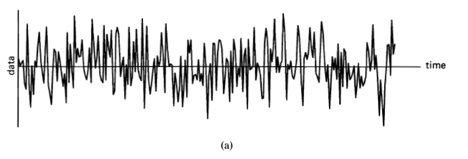
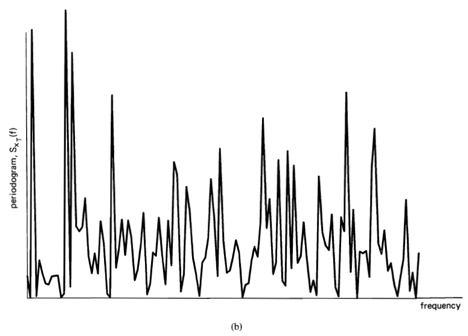
Figure 1-1 (a) Completely random data (white noise),  . (b) Periodogram of white noise, .
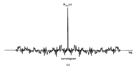
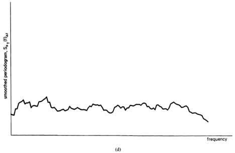
Figure 1-1 (continued) (c) Corrrelogram of white noise, . (d) Smoothed periodogram of white noise, ,  .
.
series, Wiener developed his theory of generalized harmonic analysis [Wiener 1930], in which he introduced a completely nonrandom measure of spectral content. Wiener’s spectrum can be characterized as a limiting form of an averaged periodogram. In terms of this limiting form of periodogram and the corresponding limiting form of correlogram, Wiener developed what might be called a calculus of averages for LTI transformations of time-series. Although it is not well known, 15 Wiener’s limit spectrum and its characterization as the Fourier transform of a limit
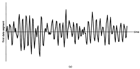
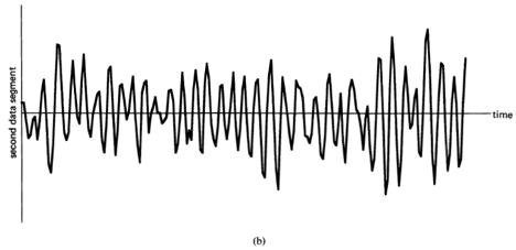
Figure 1-2 (a), (b) Two segments of narrow-band data, .
correlogram had been previously presented (in rather terse form) by Einstein [Einstein 1914].
The autonomous development of statistical mechanics, with Josiah Willard Gibbs’ (1839—1903) concept of an ensemble average, and the study of Brownian motion, by Maryan von Smoluchowski [von Smoluchski 1914], Einstein [Einstein 1906], and Wiener [Wiener 1923], together with the mathematical development of probability theory based on the measure and integration theory of Henri León Lebesgue (1875—1941) around the turn of the century, led ultimately to the probabilistic theory of stochastic processes. This theory includes a probabilistic counterpart to Wiener’s theory of generalized harmonic analysis, in which infinite time-averages are replaced with infinite ensemble averages. It greatly enhanced the conceptualization and mathematical modeling of erratic-data sources and the design and analysis of statistical data-processing techniques such as spectral analysis. The theory (for discrete-time processes) originated in the work of Aleksandr Jakovlevich Khinchin (1894—1959) during the early 1930s [Khinchin 1934] and was further developed in the early stages by Wold [Wold 1938], Andrei Nikolaevich Kolmogorov (1903—) [Kolmogorov 1941a,b], and Harald Cramér (1893—) [Cramér 1940, 1942].16 Major contributions to the early development of the probabilistic theory and methodology of statistical spectral analysis were made by Ulf Grenander and Murray Rosenblatt [Grenander and Rosenblatt 1953, 1984], Emanuel Parzen [1957a, b], and Blackman and Tukey [Blackman and Tukey 1958].
The probabilistic theory of stochastic processes is currently the popular approach to time-series analysis. However, from time to time, the alternative deterministic approach, which is taken in this book, is promoted for its closer ties with empirical reality for many applications; see [Kampé de Fériet 1954; Brennan 1961; Bass 1962; Hofstetter 1964; Finch 1969; Brillinger 1975, Sec. 2.11; Masani 1979].
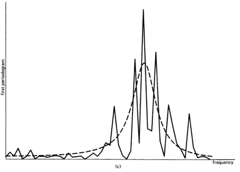
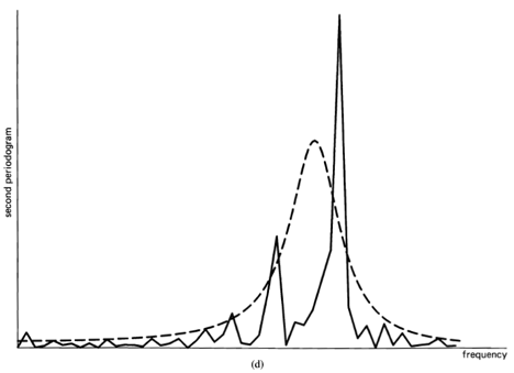
Figure 1-2 (continued) (c), (d) Periodograms of the two data segments shown in (a) and (b). (Broken curve is the limit spectrum.)
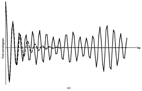
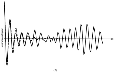
Figure 1-2 (continued) (e), (f) Correlograms of the two data segments shown in (a) and (b). (Broken curve is the limit autocorrelation.)
===============
13 See [Wiener 1938; Davis 1941; Robinson 1982] for the early history of spectral analysis. and [Chapman and Bartels 1940, Chapter XVI] for an account of early methods.
14The early history of correlation studies is reported in [Davis 1941].
15This little-known fact was brought to the author’s attention by Professor Thomas Kailath, who learned of it from Akiva Moisevich Yaglom.
16The most extensive bibliography on time-series and random processes, ranging from the earliest period of contribution (mid-nineteenth century) to the recent past (1960) is the international team project bibliography edited by Wold [Wold 1965]. Starting with 1960, a running bibliography, including abstracts, is available in the Journal of Abstracts:Statistical Theory and Method.
Section A explains that the objective of Part I of this book is to show that a comprehensive deterministic theory of statistical spectral analysis, which for many applications relates more directly to empirical reality than does its more popular probabilistic counterpart, can be (and is in this book) developed—the motivation being to stimulate a reassessment of the way engineers and scientists are often taught to think about statistical spectral analysis by showing that probability theory need not play a primary role. In Section B it is explained that the most basic purpose of spectral analysis is to represent a function by a sum of weighted sinusoidal functions called spectral components and that procedures for statistical spectral analysis average the strengths of such components to reduce random effects. It is further explained that sine wave components, in comparison with other possible types of components, are especially appropriate for analyzing data from time invariant phenomena, because sine waves are the principal components of time invariant linear transformations and because an ideal sine wave spectrum exists if and only if the data source is time-invariant (in an appropriate sense specified herein). The conceptual link between this practical empirically-motivated point of view and that of the more abstract probabilistic framework of ergodic stationary stochastic processes on which statistical spectral analysis is typically based is then explained in terms of Wold’s isomorphism. In Section C, a historical sketch of the origins of spectral analysis is presented, and finally in Section D the need for a generalization of the theory of spectral analysis of random data, from constant phenomena to periodic phenomena, is commented upon.
Appendix 1-1 is a brief review of prerequisite material on linear time-invariant transformations and the Fourier transform.
This first chapter is concluded with a brief overview of the remainder of Part I. In Chapter 2, the basic elements of empirical spectral analysis are introduced. The time-variant periodogram for nonstatistical spectral analysis is defined and characterized as the Fourier transform of the time-variant correlogram, and its temporal and spectral resolution properties are derived. The effects of linear time-invariant filtering and periodic time sampling are described. Then in Chapter 3, the fundamentals of statistical spectral analysis are introduced. The equivalence between statistical spectra obtained from temporal smoothing and statistical spectra obtained from spectral smoothing is established, and the relationship between these statistical spectra and the abstract limit spectrum is derived. The limit spectrum is characterized as the Fourier transform of the limit autocorrelation, and the effects of linear time-invariant filtering and periodic time-sampling on the limit spectrum are described. Various continuous-time and discrete-time models for time-series are introduced, and their limit spectra are calculated. Chapter 4 presents a wide variety of analog (continuous-time) methods for empirical statistical spectral analysis, and it is shown that all these methods are either exactly or—when a substantial amount of smoothing is done—approximately equivalent. The spectral leakage phenomenon is explained, and the concept of an effective spectral smoothing window is introduced. Then a general representation for the wide variety of statistical spectra obtained from these methods is—possibly for the first time—introduced and shown to provide a means for a unified study of statistical spectral analysis. In Chapter 5, it is explained that the notion of the degree of randomness or variability of a statistical spectrum can be quantified in terms of time-averages by exploiting the concept of fraction-of-time probability. This approach is then used mathematically to characterize the temporal bias and temporal variability of statistical spectra. These characterizations form the basis for an in-depth discussion of design trade-offs involving the resolution, leakage, and reliability properties of a statistical spectrum. The general representation introduced in Chapter 4 is used here to obtain—possibly for the first time—a unified treatment of resolution, leakage, and reliability for the wide variety of spectral analysis methods described in Chapter 4. Chapter 6 complements Chapter 4 by presenting a variety of digital (discrete-time) methods for statistical spectral analysis. Chapter 7 generalizes the concept of spectral analysis of a single real-valued time-series to that of cross-spectral analysis of two or more complex-valued time-series. It is established that the cross spectrum, which is a measure of spectral correlation, plays a fundamental role in characterizing the degree to which two or more time-series are related by a linear time-invariant transformation. Methods for measurement of statistical cross spectra that are generalizations of the methods described in earlier chapters are presented, and the temporal bias and temporal variability of statistical cross spectra are mathematically characterized—possibly for the first time—in a unified way based on a general representation. In Chapter 8, the application of statistical spectral analysis to time-variant phenomena is studied. Fundamental limitations on temporal and spectral resolution are discussed, and the roles of ensemble averaging and probabilistic models are described. Finally, in Chapter 9, an introduction to the theory of autoregressive modeling of time-series is presented and used as the basis for describing in an unified manner a variety of autoregressive parametric methods of statistical spectral analysis. In keeping with the theme of this book, the unification is carried out within the time-average framework, thereby avoiding the unnecessary abstraction of stochastic processes. The chapter concludes with an extensive experimental study and comparison of various parametric and nonparametric methods of statistical spectral analysis.
In Section A, the time-variant periodogram, which is the squared magnitude of the time-variant finite-time complex spectrum normalized by the data-segment length , is introduced as an appropriate measure of local spectral content of a waveform; it is established that the temporal resolution width of the time-variant periodogram is , and the spectral resolution width is on the order of . In Section B, the technique of data tapering is introduced as a means for controlling the shape of the effective spectral smoothing window in the periodogram, and several basic tapering apertures or windows are introduced. Then Section C explains that regardless of the particular tapering aperture used, the product of temporal and spectral resolution widths is always on the order of unity, because the corresponding temporal and spectral windows are a Fourier transform pair. In Section D, the time-variant correlogram is introduced as a measure of local autocorrelation of a waveform, and it is established that the time-variant periodogram is the Fourier transform of the time-variant correlogram. Then in Section E, an alternative measure of local autocorrelation termed the finite-average autocorrelation is introduced, and its Fourier transform, the pseudospectrum, is claimed to be a useful alternative to the periodogram when it is appropriately averaged to obtain a statistical spectrum. Several exact and approximate relationships among time-averaged correlograms and time-averaged finite-average autocorrelations are established for their use in the next chapter, where time-averaged measures of spectral content are studied. It is also explained that in the limit as the parameter approaches infinity both the correlogram and finite-average autocorrelation approach the ideal limit autocorrelation. In Section F, an approximate convolution relation between the correlograms (and finite-average autocorrelations) at the input and output of a filter is derived and then used to derive an approximate product relation between the corresponding periodograms (and pseudospectra). It is explained that these approximate relations become exact in the limit as the parameters in (35) and (37) and  in (39) and (40) approach infinity. These are referred to as the (input/output) limit-autocorrelation relation and limit-spectrum relation for filters, (38) and (41). In Section G, the approximate periodogram relation for filters is used to establish that the time-variant periodogram can be interpreted as a measure of local-average power spectral density only if the temporal and spectral resolutions are limited in order to satisfy the time- frequency uncertainty condition (51). Finally in Section H, the discrete-time counterpart of the continuous-time complex spectrum is introduced, and the spectral aliasing phenomenon associated with time-sampling is described. Then the discrete-time counterparts of the time-variant periodogram and time-variant correlogram are introduced, and it is established that these are a Fourier-series transform pair.
In Appendix 2-1 at the end of Chapter 2, the concept of instantaneous frequency for a sine wave with a time-variant argument is introduced and used to illustrate the resolution limitations of the time-variant periodogram.
For the sake of emphasis, two basic and fundamental results on the relationships between the overall widths and the resolution widths of Fourier transform pairs that are developed in this chapter and the exercises are repeated here at the conclusion of this summary. If a time-function has overall width (duration) on the order of , then the spectral resolution width  of its transform must be on the order of . Furthermore, if the time-function is pulselike, then its temporal resolution width
  is on the order of its overall width . Similarly, if a frequency function has overall width (bandwidth) on the order of
  , then the temporal resolution width of its inverse transform must be on the order of
  , and if the frequency function is pulselike (low-pass or band-pass) then its spectral resolution width is on the order of its overall width . These simple order-of-magnitude rules are a key to understanding the principles of spectral analysis resolution.
This chapter introduces the fundamentals of statistical spectral analysis: the equivalence between statistical spectra obtained from temporal smoothing and statistical spectra obtained from spectral smoothing, and the relationship between these statistical spectra and the abstract limit spectrum. The motivation for smoothing—to average out undesired random effects that mask spectral features of interest—is developed by consideration of the problem of measuring the parameters of a resonance phenomenon. It is established that the limit autocorrelation and limit spectrum are a Fourier transform pair and that each is a self-determinate characteristic under a linear time-invariant transformation (filtering operation). The utility of the limit spectrum for characterizing spectral features in stationary time-series is illustrated with several examples of modulated waveforms. Periodically time-sampled waveforms are considered, and a formula for the limit spectrum of the discrete-time sampled data, in terms of the limit spectrum of the waveform, is derived and used to describe further the spectral aliasing phenomenon. The moving average and autoregressive models of discrete-time data are introduced, and their limit spectra are derived. In Appendix 3-1 at the end of Chapter 3, bandpass time-series are considered and a general representation in terms of lowpass time-series is derived, and the relationships between the limit autocorrelations and limit spectra of the bandpass and lowpass time-series also are derived. In Appendix 3-2, the role of spectral analysis in the detection of random signals is explained.
In order to understand why a statistical (average) spectrum can be preferable to a nonstatistical spectrum, we must focus our attention not on the data itself but rather on the source of the data—the mechanism that generates the data. Generally speaking, data is nothing more than a partial representation of some phenomenon—a numerical representation of some aspects of a phenomenon. The fundamental reason for interest in a statistical (e.g.. time-averaged) spectrum of some given data is a belief that interesting aspects of the phenomenon being investigated have spectral influences on the data that are masked by uninteresting (for the purpose at hand) random effects and an additional belief (or, at least, hope) that these spectral influences can be revealed by averaging out the random effects. This second belief (or hope) should be based on the knowledge (or, at least, suspicion) that the spectral influences of the interesting aspects of the phenomenon are time-invariant, so that the corresponding invariant spectral features (such as peaks or valleys) will be revealed rather than destroyed by time-averaging.
This idea is illustrated with the following example. Consider the problem of determining the resonance frequency and damping ratio of a single-degree-of-freedom mechanical system (see exercise 10) that is subject to a continuous random vibrational force excitation  . The system displacement response
  can be modeled as an LTI transformation of the excitation, with the transfer function magnitude
  shown in Figure 3-1, which reveals the resonance frequency
  and the bandwidth (which can be related to the damping ratio). The vibrational response of the system is random by virtue of the randomness of the excitation. Consequently, the spectrum of the response data does not exhibit the desired single smooth peak shown in Figure 3-1. Rather, it is an erratic function with numerous sharp peaks and valleys, as revealed by the simulation shown in Figure 3-2(a). Moreover, as the time-interval of analysis is made longer by increasing , the spectrum only becomes more erratic (at least locally), as revealed by the simulation shown in Figure 3-2(b). However, if the random excitation arises from a system in statistical equilibrium, the underlying time-invariance in the excitation, as well as in the resonant system, suggests that time-averaging the response spectrum will reduce the random effects while leaving the desired spectral features intact. In fact, it is shown in the next section that for
  , the time-smoothed spectrum,
(1) ![\[ S_{y_{T}}(t, f)_{\Delta t} \triangleq S_{y_{T}}(t, f) \otimes u_{\Delta t}(t), \]](https://cyclostationarity.com/wp-content/ql-cache/quicklatex.com-8e4941eb16a047fee5fa79dbc0f1970e_l3.svg "Rendered by QuickLaTeX.com")
is closely approximated by the frequency-smoothed spectrum
(2) ![\[ S_{y_{\Delta t}}(t, f) \otimes z_{1 / T}(f), \]](https://cyclostationarity.com/wp-content/ql-cache/quicklatex.com-48b96cf7e7ccd08739bdcfa4f42e7db8_l3.svg "Rendered by QuickLaTeX.com")
and for sufficiently large and the particular form of the spectral-smoothing window  is irrelevant. Consequently, approximation (40) in Chapter 2 can be used to obtain
(3) ![\[ S_{y_{T}}(t, f)_{\Delta t} \cong|H(f)|^{2} S_{x_{T}}(t, f)_{\Delta t}}, \]](https://cyclostationarity.com/wp-content/ql-cache/quicklatex.com-41cc9f58c15ce2f65e6751a836435aa1_l3.svg "Rendered by QuickLaTeX.com")
for which it has been assumed that1
(4) ![\[ \frac{1}{T} \ll \Delta f^{*} , \]](https://cyclostationarity.com/wp-content/ql-cache/quicklatex.com-d7e6f13b8c3a40d243d6d4ed7dfa97de_l3.svg "Rendered by QuickLaTeX.com")
where is the resolution width of the function  ( is on the order of
  , where
  is the system memory length—the width of
  ). If the system excitation is completely random so that it exhibits no spectral features, then for ,
  will closely approximate a constant (over the support for which is nonnegligible), say
  . Therefore, (3) yields the desired result:
(5) ![\[ S_{y_{T}}(t, f)_{\Delta t} \cong N_{0}|H(f)|^{2}, \quad \Delta t \Delta f^{*} \geqslant \Delta t / T \gg 1, \]](https://cyclostationarity.com/wp-content/ql-cache/quicklatex.com-deb6c6e0b1e20a6297c95b80853b1bae_l3.svg "Rendered by QuickLaTeX.com")
from which the resonance frequency and damping ratio can be determined. This is illustrated with the simulations shown in Figure 3-2 (c) and (d).
In addition to illustrating the use of a statistical spectrum obtained from time-smoothing a periodogram (1), this example introduces the idea that an equivalent statistical spectrum can also be obtained from frequency-smoothing a periodogram (2). This equivalence is established in the following section. However, before proceeding it should be clarified that in practice when automated spectrum analyzers are used to study visually the spectral features of a phenomenon, it is common practice to use very little smoothing (and in some cases no smoothing) in spite of the erratic behavior of the displayed spectrum due to random effects. But it should be remembered that human visual perception incorporates spatial integration and temporal memory so that we in effect perceive a smoothed spectrum even when the analyzer uses no smoothing. This is apparent from Figure 3-2 (a) and (b), in which we can perceive the smoothed spectra that are shown in Figure 3-2 (c) and (d).
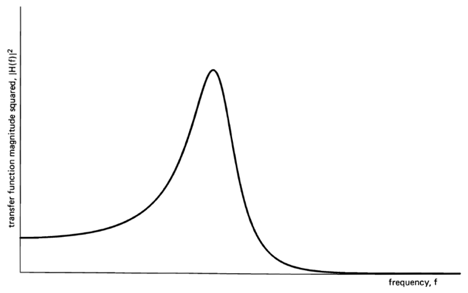
Figure 3-1 Magnitude-squared transfer function of resonant system.
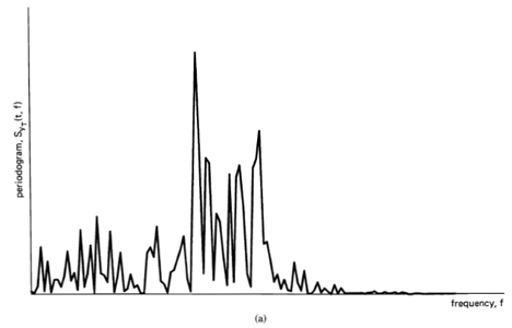
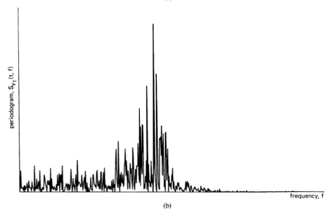
Figure 3-2 Nonstatistical spectra of response of resonant system to completely random excitation. (Length of time interval of analysis is ): (a)  , (b)
, (b)  .
.
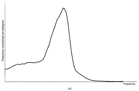
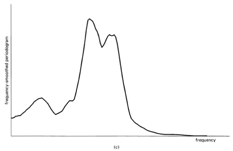
Figure 3-2 (continued) Statistical spectra obtained by frequency-smoothing the nonstatistical spectra shown in (a) and (b): (c) from (a) with  , (d) from (b) with
  .
.
===============
1Condition (4) guarantees that the order of multiplication with and convolution with
  in(40), Chapter 2, can be interchanged to obtain a close approximation.
In the spectral analysis problem considered in Section A, the spectral features of interest as described by can be measured only approximately with a finite amount, , of data, as indicated by approximation (5). But as shown in subsequent sections, can be determined exactly in the abstract limit as  , as indicated by (28) and (38). This reveals that exact description of the spectral characteristics of a phenomenon requires an abstract mathematical model for the data, namely, the limit spectrum.
We have thus arrived at the point of view of statistical inference, which is that an abstract mathematical model is the desired result that can be only approximately discovered (inferred) with the use of a finite amount of data.
From the point of view of statistical inference, the object of statistical spectral analysis is spectrum estimation, by which is meant estimation of the limit spectrum.13 Succinctly stated, the classical spectrum estimation design problem is: given a finite amount14 of data, determine the best value of spectral resolution  to obtain the best estimate of
  . This involves a trade-off between maximizing spectral resolution, which corresponds to minimizing and minimizing the degree of randomness or variability (described in Chapter 5), which in turn corresponds to maximizing in order to maximize the product
  .
.
The statistical-inference or spectrum-estimation interpretation given here to spectral analysis is unconventional in that it does not rely on probabilistic concepts.
However, it can be put into a probabilistic framework by reinterpreting infinite time averages as ensemble averages (expectations) via H. O. A. Wold’s isomorphism (defined in Chapter 1, Section B). This is done in Chapter 5, where the notion of degree of randomness is quantified in terms of a coefficient of variation that is shown to be inversely proportional to the resolution product .
As a matter of fact, the classical spectrum estimation design problem is more involved than suggested by the preceding succinct statement, because the shape as well as the width of the effective spectral window should be optimized in order to minimize the undesirable spectral leakage effect. This effect is described in the next chapter, and the design problem that simultaneously takes into account resolution, leakage, and degree of randomness is explained in Chapters 5 and 6.
Before proceeding, a few words about the notion of degree of randomness will be helpful to tide us over until the subject is taken up in Chapter 5. It has been shown in this chapter that randomly fluctuating (in both and ) statistical spectra, such as  and
and  , converge in the limit (,
  ) to the nonrandom limit spectrum if the limit autocorrelation exists, which is necessary for a constant phenomenon. The degree of randomness or variability of a statistical spectrum can be interpreted as the degree to which the statistical spectrum varies from one point in time to another. If the underlying phenomenon is indeed constant, as hypothesized in Part I, then fluctuation with time of the statistical spectrum must be attributed to random effects. it is shown in Chapter 5 that the time-averaged squared difference between statistical spectra measured at two different times separated by an amount
  , for example, is approximately inversely proportional to the resolution product (for sufficiently small and sufficiently large ) for all
  . Also, the time-averaged squared difference between the statistical spectrum and the nonrandom limit spectrum behaves in the same way. Thus, this temporal mean-square measure of the degree of randomness of a statistical spectrum reveals that the degree of randomness is made low (or the reliability is made high) by making the resolution product large.
This central characteristic of statistical spectral analysis has been arrived at without resorting to the mathematical artifice of pretending the data is one member of an ensemble corresponding to a stochastic process, and then interpreting degree of randomness as variability over the make-believe ensemble—which is a huge departure from empirical reality.
This key result exposes the confusion that reigns in efforts to understand empirical data in terms of the unnecessary theory of stochastic processes.
Note dated June 2020: The several negative reviews of this book written within a few years of its publication in 1987 and at strong odds with the positive reviews clearly reveal this common state of confusion even among experts judged worthy of reviewing technical books. (See page 3.3 of this website.)
===============
13In the literature, the terms spectrum analysis and spectral estimation are often used in place of the terms spectral analysis and spectrum estimation, which are used in this book, the latter two terms are more appropriate since we are not concerned with analysis of a spectrum but rather with analysis of data into spectral components, and we are not concerned with estimation using spectral methods but rather with estimation of a spectrum. Nevertheless, because of the long-standing tradition of referring to spectral analysis instruments as spectrum analyzers, this term is used in this book in place of the term spectral analyzers.
14 The actual amount of data needed to average a periodogram of length  over an interval of length is
  , but this is closely approximated by for
  .
.
In Section A, the problem of measuring the parameters of a resonance phenomenon from the randomly resonant response to random excitation is considered in order to motivate consideration of averaging methods for reducing random effects. It is explained that from the point of view adopted here, we focus attention on the phenomenon that gives rise to random data rather than on the data itself, and we apply averaging methods to the nonstatistical spectrum (periodogram) of the data to obtain a statistical spectrum in which the random effects in the data that mask the spectral influences from the phenomenon are reduced. In Section B, a profound fundamental result establishing an equivalence between time-smoothed and frequency-smoothed periodograms is developed. This equivalence reveals that the periodogram of the data-tapering window in a temporally smoothed periodogram of the tapered data is an effective spectral smoothing window in an equivalent spectrally smoothed periodogram of the untapered data. Then in Section C, the idealized limiting form of the statistical spectrum with and (in this order) is shown to be simply the Fourier transform of the limit autocorrelation. This characterization of the limit spectrum, called the Wiener relation, is used to derive the limit-spectrum relation for filters (28), which in turn is used to establish the interpretation of the limit spectrum as a spectral density of time-averaged power.
In Section C, several signal and noise models are introduced, and their limit spectra are calculated. Then in Section D, the definition of the limit spectrum is adapted to discrete-time data by simply replacing the Fourier transform with the Fourier-series transform introduced in Section H of Chapter 2. A spectral aliasing formula relating the limit spectra of a waveform and its time-samples is derived. In Section F, three basic time-series models for discrete-time data are introduced. These are the MA, AR. and ARMA models. Formulas for the limit spectra for these models are derived in terms of the parameters of the models.
Finally in Section G, it is pointed out that the arguments presented in the beginning of this chapter have led us to the point of view of statistical inference. which is that an abstract mathematical model—the limit spectrum in this case— is the desired result that can be only approximately discovered (inferred) with the use of a finite amount of data. Thus statistical spectral analysis is typically called spectrum estimation. This section ends with a brief discussion of the dependence of the degree of randomness or variability of a statistical spectrum on the resolution product .
In Appendix 3-1 at the end of Chapter 3, Rice’s representation is derived. This provides a means for representing band-pass waveforms in terms of low-pass waveforms. Then the limit spectra for the low-pass representors are characterized in terms of the limit spectrum of the band-pass waveform, and vice versa. In Appendix 3-2, the problem of detecting the presence of a random signal in additive random noise is considered, and the central role played by the periodogram and the limit spectrum is revealed.
In Chapter 3 it is established that a statistical spectrum can be obtained from a periodogram by either the temporal-smoothing method or the spectral-smoothing method and that these two methods yield approximately the same statistical spectrum when a substantial amount of smoothing is done (). In this chapter it is shown that a variety of alternative methods yield approximately or exactly the same statistical spectrum, but it is emphasized that differences can be quite important in practice. These alternatives include the methods of temporal or spectral smoothing of the pseudospectrum, hopped temporal smoothing of the periodogram and pseudospectrum, Fourier transformation of the tapered correlogram and finite-average autocorrelation, real and complex wave-analysis, real and complex demodulation, and swept-frequency-demodulation wave-analysis. The methods are referred to as analog methods because they process the continuous-time waveforms directly. The actual form of implementation of such methods can employ conventional resistive-capacitive-inductive passive electrical circuits, more modern active electrical circuits, microwave devices, various optical, acousto-optical, and electro-acoustical devices, or mechanical devices. The particular form of implementation depends on available technology, economic constraints, environmental constraints (e.g., temperature, mechanical vibration, humidity, and so on), and frequency ranges of interest. The upcoming Chapter 6 presents digital methods, so called because they process discrete-time data and because digital electrical forms of implementation (both hardware and software) are the primary means for discrete-time processing.
In this chapter, an introductory comparative study of a variety of analog (continuous-timeand continuous-amplitude) methods of measurement of statistical spectra is conducted. In Section A, approximate equivalences among the four methods based on temporal and spectral smoothing of the penodogram and pseudospeetrum are derived, and in Section B it is established that the two spectral smoothing methods are each exactly equivalent to a method consisting of Fourier transformation of a tapered autocorrelation function. The resultant eight distinct methods for obtaining the four distinct (but approximately equivalent) statistical spectra are summarized in Figures 4-1 and 4-2 (see below). In Section C, the spectral leakage phenomenon that results from the sidelobes of the effective spectral smoothing window is explained, and the sine-wave-removal, tapering, and prewhitening approaches to reducing spectral leakage are described. Then Section D explains that temporal smoothing based on continuously sliding periodograms or pseudospectra can be modified to obtain hopped periodograms or pseudospectra, and an exact equivalence between a hopped time-averaged pseudospectrum and a spectrally smoothed pseudospectrum is derived. A similar but approximate equivalence for the hopped time-averaged penodogram is derived in exercises I and 2.
In Section E, an alternative method for implementing the temporally smoothed periodogram, which is based on filtering is introduced. Both real and complex implementations, called wave analyzers, are developed (Figure 4-4, see below). Then in Section F, another alternative implementation based on demodulation is derived. The real and complex implementations of the demodulation spectrum analyzer (Figure 4-6, see below) can be obtained directly from the corresponding implementations of the wave analyzer by using band-pass-to-low-pass transformations on the filters (Figure 4-8). It is then explained that an economical way to construct a spectrum analyzer that covers a broad range of frequencies is to use the demodulation method and sweep the frequency of the sine wave used for demodulation. It is also explained that it is often more practical to use swept-frequency demodulation to down-convert all frequencies to a fixed nonzero intermediate frequency and then use the wave-analysis method (Figure 4-7, see below). In addition, an alternative method of swept-frequency spectral analysis that incorporates time compression is described in exercise 14.
Finally in Section G, a general representation for all preceding types of spectrum analyzers (except the swept-frequency wave analyzer) is introduced, possibly for the first time, and it is explained that the two width parameters and of the kernel  that prescribes the representation for a particular spectrum analyzer determine the temporal and spectral resolution widths of the statistical spectrum produced by the analyzer. A convenient separable approximation (75) to the kernel is introduced, and it is explained that the resultant approximate and exact general representations provide a unifying basis for the design and analysis of spectrum analyzers. This is demonstrated in the next chapter.
In Appendix 4-1 at the end of Chapter 4, an alternative wave-analysis method that is equivalent to a method based on Fourier transformation of a tapered autocorrelation is presented.
In this chapter the concept of fraction-of-time probabilistic analysis is introduced and used to quantify the resolution, leakage, and reliability properties of statistical spectra. In Section A it is explained that probabilistic analysis can be carried out without relying on the abstract notion of a probability space and an associated ensemble of random samples by using the concept of fraction-of-time probability. Then in Section B, the general fraction-of-time probabilistic model is defined and the particularly important special case, the Gaussian model, is defined. In Section C, the two temporal probabilistic measures of performance called bias and variability are defined and characterized in terms of the temporal mean, temporal coefficient of variation, and temporal correlation coefficient. These temporal probabilistic parameters are evaluated for the complex spectrum, periodogram, and various statistical spectra specified by the general representation introduced in Chapter 4, Section G. A general formula (50) – (51)for the effective spectral smoothing window is obtained and evaluated for various specific types of statistical spectra. A general formula (72) – (73) for the coefficient of variation is obtained, and it is simplified ((74) – (77)) by using the separable approximation to the kernel in the general representation (48), and the variability phenomenon is explained. Then two examples that illustrate the effects of variability are presented, and a time-frequency uncertainty principle for statistical spectra is described. Finally, the utility of the explicit formula for the effective spectral smoothing window is brought to light by explaining how it can be used in design to trade off resolution, leakage, and reliability performance (see Table 5-2). Two examples are presented to illustrate these design trade-offs. For situations in which the amount of data available is severely restricted or the range of the spectrum is large, such that the conditions required for the approximate formula for the coefficient of variation to be accurate are violated, the exact formulas for the mean (50) – (51) and variance (66) can be used simply by substituting in the kernel  that specifies the particular spectrum estimate of interest (see Table 5-1). This is important because leakage effects that do not show up in the effective spectral smoothing window can be revealed in the variability when the exact formulas are used.
Modern general-purpose spectral analysis instruments are typically implemented using primarily analog technology for frequencies above 100 KHz and digital technology for frequencies below 100 Hz, and both technologies are used in the midrange. The swept-frequency method described in Chapter 4 is the most commonly used analog method for general-purpose instruments, whereas the fast Fourier transform (FFT), with the discrete-time and discrete-frequency counterparts of the frequency smoothing and/or hopped time-averaging methods described in Chapter 4, is used for most digital implementations. Digital methods are especially attractive for low frequencies because the most attractive analog method (swept frequency) requires long measurement times compared with the simultaneous analysis methods based on Fourier transformation of the data. Analog methods are especially appropriate for high frequencies because of technological limitations on switching times, which limit the speed of digital computation. When the required speed is not a limiting factor, digital implementations are generally attractive because of economy as well as high accuracy, stability, and flexibility, including programmability. Furthermore, spectral analysis at frequencies far above 100 KHz can be accomplished digitally by down-converting spectral bands (of width less than 100 KHz) from higher frequency ranges (e.g., megahertz to gigahertz) to lower frequency ranges (below 100 KHz), and this band-selective approach can be used to obtain very high spectral resolution. Moreover, the flexibility of digital methods is an attractive feature for many special-purpose spectral analysis tasks, where general-purpose instruments are inappropriate. An example of this flexibility is the fact that digital methods can be directly implemented in software so that both the convenience of personal computers and the immense data-handling capabilities of supercomputers are available for spectral analysis. Finally, because of the increasing amount of data that is digitally encoded for storage and transmission, digital methods of spectral analysis that can be directly applied to digital data are especially appropriate.
Unfortunately, the study of digital methods of spectral analysis is somewhat more complicated than the study of analog methods for several reasons. These include 1) the spectral aliasing phenomenon that results from time-sampling. 2) the discrete nature of the frequency parameter in FFT and other discrete Fourier transform (DFT) algorithms, and 3) the block format for data that is required by DFT algorithms. All three of these items are sources of conceptual complication that can lead to complications in practice, including erroneous procedures and misinterpretation of results. Fortunately, many of the fundamentals of spectral analysis can be understood, as explained in the other chapters of this book, without introducing the complications associated with digital methods of implementation. This applies especially to the digital methods of spectral analysis that are simply discrete-time and discrete-frequency counterparts of the analog methods studied in Chapter 4.
In Section B, the DFT is introduced and its properties and relationships with other Fourier transformations are studied. Then in Section C, various digital counterparts of the analog methods developed in Chapter 4 are described. Finally in Section D, the applicability to discrete-time spectrum estimates of the results on fraction-of-time probabilistic analysis obtained in Chapter 5 for continuous time is explained.
In Section A, the complementary nature of analog and digital methods of spectral analysis are discussed. Then in Section B the DFT, on which most digital methods are based, is studied. Topics include the use of zero-padding to control resolution, the distinction between circular and linear convolutions, the circular convolution theorem and the associated wraparound phenomenon, and a circular correlogram-periodogram relation. Also, the relationships among the DFT, FST, and CFT are described, and the importance of zero-padding is discussed and illustrated by example. In Section C various digital methods for statistical spectral analysis that are based on the DFT are described and compared. It is explained that these methods, known by the names Bartlett-Welch, Wiener-Daniell, Blackman-Tukey, and channelizer methods, are all digital counterparts of analog methods studied in Chapter 4. Then the minimum-leakage method, which is an optimized wave analyzer (channelizer), is derived and its interpretation in terms of maximum likelihood is explained. Finally in Section D, it is explained that the formulas derived in Chapter 5 for the mean and variance of continuous-time spectrum estimates apply equally well to discrete-time spectrum estimates, provided only that the range of integration over frequency variables is reduced from  to [˗½, ½], to reflect the replacement of the CFT by the FST in the derivation.
In this chapter, the concept of the spectral density of a single real-valued time-series is generalized to the concept of the cross-spectral density of two complex-valued time-series. Complex-valued time-series are considered in order to accommodate complex low-pass representations of real band-pass time-series (see Appendix 3-1). It is established that the cross spectrum, which is a measure of spectral correlation, plays a fundamental role in characterizing the degree to which two time-series are related by a linear time-invariant transformation. Methods for measurement of statistical cross spectra that are straightforward generalizations of the methods described in Chapter 4 for measurement of statistical spectra are described. The chapter concludes with a discussion of the resolution, leakage, and reliability properties of cross-spectrum measurements. Three appendices describe applications of cross-spectral analysis to propagation path identification, distant source detection, and time- and frequency-difference-of-arrival estimation.
As explained in Chapter 4, statistical spectral measurements can be obtained from any of a variety of methods, and these various methods are either exactly or approximately equivalent to each other. In principle, the approximations can be made as accurate as desired by choosing sufficiently large provided only that the limit autocorrelation exists. In particular, there are more than 10 alternative methods, which are described by diagrams in Figures 4-1, 4-2, 4-4, 4-6, and 4-7. Because of the fact that all the elements of cross-spectral analysis are straightforward generalizations of the elements of spectral analysis, as explained in Section A, all these alternative methods for obtaining statistical spectra generalize in a straightforward way for statistical cross spectra. Some of these generalizations are briefly described in this section. As explained in Chapter 4, Section A, although the approximations relating the spectra obtained from these various methods can in principle be made as accurate as desired by choosing sufficiently large, it should be emphasized that in applications where must be relatively small, the differences among statistical spectra obtained from different smoothing methods or different windows can he substantial, and the particular choice then becomes an important component of the design problem, as illustrated in Chapter 5,Section D. Although only analog methods are described here, the corresponding digital methods can easily be deduced from these and the digital methods based on the DFT described in Chapter 6, Section C.
In Section A, the elements of cross-spectral analysis are introduced, and it is explained that these are all generalizations of the elements of spectral analysis. These elements include the cross periodogram, cross correlogram, finite-average cross correlation, pseudo-cross spectrum, limit cross correlation and limit cross spectrum, and the various temporally smoothed and spectrally smoothed statistical cross spectra. It is also explained that whereas the limit spectrum gives the mean-square strength of spectral components, the limit cross spectrum gives the correlation of spectral components in two distinct time series. In Section B. the spectral coherence function, which is the spectral correlation coefficient obtained from the limit cross spectrum, is introduced and is shown to be a measure of the degree to which two time-series are related by a linear time-invariant transformation. The two extremes of completely coherent and completely incoherent time-series are described, and the role of coherence in the identification of dynamical systems is explained. Then the concept of coherence is generalized to that of partial coherence for a pair of time-series that are coherent with other time-series. In Section C, the central role of spectral correlation (coherence) in the spectral analysis of random data from periodic phenomena is explained, and the spectral autocoherence function for a single time-series is defined, and is illustrated for a class of amplitude- and phase-modulated sine waves.
In Section D. the various analog methods for statistical spectral analysis that are described in Chapter 4 are generalized for statistical cross-spectral analysis. This includes the methods of temporal and spectral smoothing, Fourier transformation of tapered cross correlations, cross-wave analysis, and cross demodulation (see Figures 7-1, 7-2, 7-3 below). In Section E, the results on resolution, leakage, and reliability that are developed in Chapter 5 for spectral analysis are generalized for cross-spectral analysis, and it is explained that the variability and resolution of cross-spectrum estimates can be even more problematic than for (auto) spectrum estimates.
Appendix 7-1 describes the use of cross-spectral analysis for propagation path identification. Appendix 7-2 explains the use of cross-spectral analysis for distant-source detection. Appendix 7-3 reveals the connection between the cross-correlation function, the cross-spectral density function, and the cross-ambiguity function for the problems of time- and frequency-difference-of-arrival estimation.
As explained in Chapter 1, spectral analysis is especially appropriate in principle only for time-invariant linear transformations of data and for data from time-invariant phenomena. But, from a pragmatic point of view, we expect spectral analysis to be useful for time-variant linear transformations and for data from time-variant phenomena, provided that time variation is sufficiently slow. The purpose of this chapter is to clarify why time variation must be slow and how slow it must be. Only the situation in which the time-series data alone is to be used for spectral analysis is considered. That is, the model-fitting methods described in Chapter 9, which typically require additional information for the purpose of model-type selection, are omitted from consideration.
Regardless of the phenomenon or the data under study, the time-variant periodogram introduced in Chapter 2, Section A, is the normalized squared magnitude of a time-variant density of spectral components (namely, the time-variant finite-time complex spectrum; see (2b) in Chapter 2), and is therefore the most natural definition and the only generally appropriate definition of a nonstatistical time-variant spectrum. As explained in Chapter 5, Section C, if there is no ensemble of time-series available from the phenomenon of interest, then the degree of randomness of this spectrum can be reduced (reliability increased) only by temporal or spectral smoothing, with the result that temporal and spectral resolution are severely constrained by Grenander’s uncertainty condition, (89) in Chapter 5,
(1) ![\[ \Delta t \Delta f \gg 1, \]](https://cyclostationarity.com/wp-content/ql-cache/quicklatex.com-a1e7a92f4c30bc1ac9df0f7d4639cc0e_l3.svg "Rendered by QuickLaTeX.com")
which is a necessary and sufficient condition (for a broad class of time-series data) for high reliability. Thus, the reliable resolvability of time variation in spectral characteristics of a phenomenon is limited by a temporal resolution width that must greatly exceed the reciprocal of the spectral resolution width . On the other hand, if an ensemble of replicas of a time-series (not timetranslates of a single time-series but rather genuine random samples as would be obtained, for example, from replicating an experiment) from a given timevariant phenomenon is available, then as explained in Chapter 5, Section A, the degree of randomness can be reduced by ensemble averaging with no degradation in either temporal or spectral resolution. Thus, resolvability is limited by only Gabor’s uncertainty principle, (88) in Chapter 5,
(2) ![\[ \Delta t \Delta f \cong 1, \]](https://cyclostationarity.com/wp-content/ql-cache/quicklatex.com-8f2198da8ecc89971bff48754b199734_l3.svg "Rendered by QuickLaTeX.com")
which applies to the time-variant periodogram, whether or not it is ensemble averaged. Furthermore, even when an ensemble is not physically available, the concept of an ensemble-averaged time-variant spectrum can be of value.1 Specifically, the idealized limit of an ensemble-averaged time-variant periodogram, (4) in Chapter 5, which is the expected time-variant periodogram
(3) ![\[ \mathcal{S}_{x_{T}}(t, f) \triangleq E\left\{S_{x_{T}}(t, f)\right\} \]](https://cyclostationarity.com/wp-content/ql-cache/quicklatex.com-4a1f5e67303df5a9d4f33d5444b2e7b0_l3.svg "Rendered by QuickLaTeX.com")
can be interpreted as a completely reliable (zero degree of randomness) measure of the time-variant spectral characteristics of a phenomenon. This most reliable measure exhibits the best possible temporal and spectral resolutions, that is, the resolutions satisfy (2). From this point of view, it apparently makes no sense to conceive of or seek a probabilistic measure of time-variant spectral characteristics that exhibits finer resolutions than those that satisfy (2).
Nevertheless, there is a probabilistic function of time and frequency that plays a fundamental role in the mathematical characterization of the expected periodogram  and that is not subject to any counterpart of (2). Specifically, it can be shown (exercise 1) [Mark 1970], that the expected periodogram is a time- and frequency-smoothed version of a function called the probabilistic instantaneous spectrum,
(4) ![\[ \mathscr{S}_{x_{T}}(t, f)=\int_{-\infty}^{\infty} \int_{-\infty}^{\infty} S_{x_{T}}(t-\tau, f-v) w(\tau, v) d \tau d v \]](https://cyclostationarity.com/wp-content/ql-cache/quicklatex.com-f226df15cb0738c3db408ece91e9bfaa_l3.svg "Rendered by QuickLaTeX.com")
in which the smoothing function is defined by
(5) ![\[ w(\tau, v) \triangleq \frac{1}{T} \int_{-\infty}^{\infty} T u_{T}\left(\tau+\frac{u}{2}\right) T u_{T}\left(\tau-\frac{u}{2}\right) e^{-i 2 \pi v u} d u \]](https://cyclostationarity.com/wp-content/ql-cache/quicklatex.com-2e20cf012c703314444047f5718b9081_l3.svg "Rendered by QuickLaTeX.com")
and the probabilistic instantaneous spectrum  is defined by
(6) ![\[ \mathcal{S}_{x}(t, \cdot) \triangleq F\left\{\mathcal{R}_{x}(t, \cdot)\right\} \]](https://cyclostationarity.com/wp-content/ql-cache/quicklatex.com-df67e08e09e27de947b2eb9de237070a_l3.svg "Rendered by QuickLaTeX.com")
(7) ![\[ \mathcal{R}_{x}(t, \tau) \triangleq E\left\{x\left(t+\frac{\tau}{2}\right) x\left(t-\frac{\tau}{2}\right)\right\} \]](https://cyclostationarity.com/wp-content/ql-cache/quicklatex.com-01da5d99fa8ba5d3a3c7ea9af521c5ba_l3.svg "Rendered by QuickLaTeX.com")
where  is called the probabilistic instantaneous autocorrelation function. Although the probabilistic instantaneous spectrum can in principle be measured as accurately as desired when a sufficiently large ensemble is physically available, in general it does not represent a time-variant spectrum of the data in any physical sense.2 It can only approximate a time-variant spectrum, and this approximation can be close only when the time-variation is sufficiently slow that the fine structure of the function is accurately resolved with resolution widths satisfying
(8) ![\[ \Delta t \Delta f \geqslant 1 \]](https://cyclostationarity.com/wp-content/ql-cache/quicklatex.com-2920ab18dbbf923fecfcf7aeb43d17ae_l3.svg "Rendered by QuickLaTeX.com")
(see [Mark 1970; Donati 1971]). But it can be shown by using (4)-(5) that when (8) is satisfied, then (using  )
)
(9) ![\[ \mathcal{S}_{x_{T}}(t, f) \cong \mathcal{S}_{x}(t, f). \]](https://cyclostationarity.com/wp-content/ql-cache/quicklatex.com-1729687a2fd79a47476733373cc2579e_l3.svg "Rendered by QuickLaTeX.com")
As a reflection of the facts stated in the preceding discussion, the expected time-variant spectrum is called the physical spectrum to distinguish it from the generally nonphysical instantaneous probabilistic spectrum [Mark 1970; Eberly and Wodkiewicz 1977].
===============
1 Wold’s isomorphism cannot be used to envision an appropriate ensemble in this case, as done in Chapter 5, Section B for time-invariant phenomena, because the equivalence between ensemble- and time-averaging would result in all time variation being averaged away by the ensemble averaging operation.
2 However, it is explained in Part II that for a cyclostationary or almost cyclostationary process, the Fourier coefficients of the periodic or almost periodic function  are spectral correlation functions, which do indeed have a concrete physical interpretation.
In Section A the fundamental limitations on the simultaneous temporal and spectral resolution capabilities of statistical spectra are described, and the advantage of ensemble averaging (when possible) is explained. The instantaneous probabilistic spectrum is introduced and its relation to the physical spectrum is explained and illustrated with an application to the problem of identification of a time-variant linear system. An alternative to the instantaneous probabilistic spectrum as an idealized probabilistic time-variant spectrum, called the evolutionary spectrum, is introduced and its direct relationship with the system function is explained. The limitations on measurement of these idealized probabilistic spectra, when ensemble averaging cannot be used, are explained and the concepts of locally stationary and locally ergodic processes are introduced.
In Section B the fact that a periodically time-variant phenomenon is an exceptional case is briefly discussed. It is explained that for this special type of time-variant phenomenon, the fundamental resolution limitations do not apply. Another exception also should be mentioned: those situations in which the spectral analyst has more information about the phenomenon under study than can be obtained from the time-series alone. For example, if it is known that the time-series can be accurately modeled as an autoregression, then—as explained in Chapter 9—spectral resolution performance that exceeds that of the periodogram is possible (but is not guaranteed).
A general treatment of the related problem of reliable measurement of time-variant auto- and cross-correlation functions is given in [Gardner 1987c].
All the methods of spectral analysis described in previous chapters are based on a direct decomposition of the data to be analyzed into spectral components using Fourier transformation or filtering and are therefore called direct methods. In contrast, the methods studied in this chapter are based on an entirely different philosophy. Specifically, each of these methods fits a particular form of model to the data by adjusting the values of parameters in the model. Once the model fitting is complete, the parameter values can be substituted into a formula to obtain the limit spectrum for that model with the estimated parameter values. There are many variations on this prototypical method. All such methods are referred to as parametric methods, whereas the direct methods described in previous chapters based on direct decomposition into spectral components are referred to as nonparametric methods.
Parametric methods of spectral analysis can yield better resolution of multiple spectral lines or other narrow features, particularly if they are close together in frequency, when the amount of data is severely limited, especially if the data-segment length is smaller than the reciprocal of the desired spectral resolution, and the experiment is repeatable so that an ensemble of data segments is available. (This occurs, for example, in some sensor-array signal-processing problems, where the spatial data-segment length is the number of sensors and ensemble averaging is performed by time-averaging.) But more generally the relative advantages depend on the appropriateness of the form of the model chosen. In some cases, nonparametric methods are helpful in selecting a form of model to be used as the basis for a parametric method. In fact, in some applications the main objective is to fit a model to the data, and nonparametric spectral analysis methods are often used as a first step. But, even when an appropriate form of model for a signal is known, if the signal is masked by noise, then nonparametric methods can be superior for spectral analysis. However, parametric methods can be particularly useful for identification (detection and estimation) of additive sine wave components to be removed (to minimize spectral leakage) before application of a nonparametric method. Generally speaking. parametric methods are more computationally burdensome than nonparametric methods, but some methods based on autoregressive models are computationally competitive with direct methods based on the FFT. The practicality of autoregressivemodel-fitting methods of spectral analysis is attested to by the wide range of problems to which these methods have been applied. These include radar, sonar, image processing, radio astronomy, biomedicine, speech analysis and synthesis, geophysics, seismology, and oceanography.
Since parametric methods of spectral analysis are diverse and often tailored to special types of data, it is not possible to present a comprehensive and unified treatment paralleling that presented in previous chapters for the direct methods. However, the fundamental concepts and mathematical theory underlying the particularly important class of autoregressive methods can be and therefore are presented in a unified manner. In keeping with the philosophy of this book, the unified treatment is non-probabilistic, whereas other treatments of the same material are typically couched within the conventional probabilistic framework. This is possibly the first time a unified theoretical treatment of this class of methods, without the use of the abstract stochastic process framework, has been presented.
Although the results of the fraction-of-time probabilistic analysis, such as bias and variance formulas derived in Chapter 5, apply to all direct methods, the parametric methods are not amenable to such straightforward probabilistic analysis—fraction-of-time or stochastic. Useful results on bias and variance are typically obtainable only asymptotically as the data segment length used for spectral analysis approaches infinity (see [Kay 1987]), and such results have typically been derived only within the abstract stochastic process framework for no special reason I can discern other than ignorance of the fraction-of-time theory presented in the book [Bk2] and now this website.
In Section B, the non-stochastic theoretical background for autoregressive and related ARMA methods is presented. Then, in Sections C and D some of the methods that have proven to be of practical value are described. Finally, in Section E, an extensive experimental study and comparison of these and direct methods is presented. The reader is cautioned that the term non-probabilistic used frequently in this chapter and elsewhere in the book, usually means non-stochastic. In many cases of this usage herein, the quantities or modeling methods referred to are based on time averages but admit a fraction-of-time probabilistic interpretation as explained in Chapter 5.Thus, strictly speaking, they are temporally-probabilistic but non-stochastic. This point is often a conceptual stumbling block for readers who are familiar with the conventional stochastic-process theory and are looking for a flaw in this author’s thinking that would justify their dismissal of the alternative theory presented herein despite its considerable advantages. Unfortunately, such biased readers all too often appear to think they’ve found a flaw and believe this author has resorted to slight-of-hand to dismiss troublesome aspects of the non-stochastic approach. This author writes extremely carefully and the likelihood of their being flaws in the logic or any devious methods of tricking the reader is near zero.
All the direct methods of spectral analysis described in preceding chapters yield spectrum estimates of the MA type except for the minimum-leakage method, which yields spectrum estimates of either the AR or ARMA types and generally provides better resolution of sharp spectral peaks. It has been reported that of the four AR LS methods, the best resolution of sharp peaks using short data-segment lengths is provided by the FB method, the poorest (relatively speaking) is provided by the YW method, and the Burg method does somewhat better than the covariance method. But there are many other performance criteria to be considered when selecting a method in practice. For example, both the YW and Burg methods guarantee a stable AR model, whereas neither the covariance nor FB LS methods guarantee stability, although in practice they typically do yield stable models, and even an unstable model can produce a useful spectrum estimate. The variance of the minimum-leakage AR method is reportedly smaller than that of the YW method [Baggeroer 1976], but the YW method has smaller variance than both the covariancc method and the Burg method for short data segments; the FB LS method has been said to have the smallest variance (as well as the best resolution) of all the LS AR methods [Swingler 1974; Ulrych and Bishop 1975; Nuttal 1976; Ulrych and Clayton 1976] but the minimum-leakage method can be superior as illustrated in Section E. Also, for sine waves in additive broadband noise, the YW, covariance, and Burg methods all occasionally produce two close spectral peaks around the frequency of a single sine wave (the spectral line-splitting phenomenon), but the FB LS method [Kay and Marple 1981] and the modified (weighted) Burg method [Helme and Nikias 1985], [Paliwal 1985] have not been observed to do this. Moreover, the location of the peaks in these latter two methods are generally closer to the correct frequencies than in the other three LS AR methods [Kay 1987]. It is also of interest that in all four LS AR methods, the amplitude of a spectral peak is proportional to the square of the power in the underlying spectral line associated with a sine wave for high signal-to-noise ratio, but the area under the peak is proportional to the power (because the width is inversely proportional to the power) [Lacoss 1971]. On the other hand, the amplitude of a spectral peak produced by the minimum-leakage AR method is indeed proportional to the power [Lacoss 1971] (assuming that the width of the spectral line is narrower than the effective resolution width for this method) as it is for all the direct methods. In summary, it appears that the best performing LS AR methods for sharply peaked spectra are the FB LS method and the modified Burg method. It should also be noted that additive white noise in the data generally has a smoothing effect on these AR spectrum estimates. Consequently, for sufficiently low signal-to-noise ratio sine waves in noise, the resolution performance of all these LS AR methods becomes inferior to that of the direct methods [Kay 1987]. (Also, for MA-type time-series, AR methods can be substantially inferior to direct methods [Beamish and Priestley 1981].) Nevertheless, other AR methods, such as the ODNE and SVD methods can reportedly provide improved performance for some low signal-to-noise ratio (e.g., as low as 0 dB) applications [Cadzow 1982; Tufts and Kumaresan 1982; Cadzow et al. 1983]. These SVD methods also considerably improve on other related but earlier parametric methods designed specifically for sine waves in noise, such as the Hildebrand-Prony method and the Pisarenko method (see [Tufts and Kumaresan 1982; Kay 1987]).
Another performance criterion to consider in selecting a method for spectral analysis is the ease with which spectrum estimates can be updated as time passes in applications where it is desired to do time-variant spectral analysis. Updating is relatively straightforward for direct methods, as explained in Chapter 6, and is also possible for many of the AR methods but is not quite as simple [Friedlander 1982a, 1982b, 1983a, 1983b; Cioffi and Kailath 1984; Honig and Messerschmitt 1984; Marple 1987]. It should be emphasized that the focus on computationally efficient methods of spectral analysis is appropriate in situations where large amounts of data are continually produced, such as in radar, sonar, and seismology signal-processing applications. However, in situations where the cost or other limitations on collecting data are dominant, this focus is not necessarily appropriate, and the more computationally burdensome but potentially higher-performing exact or near-exact maximum-likelihood methods can be attractive. This is especially true for ARMA methods, which are discussed in the next section.
Finally, it should be emphasized that the appropriateness of parametric methods for sharply peaked spectra applies only when there are multiple peaks that are closely spaced. If the separation between peaks exceeds the resolution width  determined by the amount of data available, then direct non- parametric methods typically perform just as well, if not better. In fact it is shown in exercise 22 that for a spectrum with a single sharp peak, modeled by a time-series consisting of a single sine wave in additive white Gaussian noise, the periodogram provides optimum (maximum-likelihood) estimates of the amplitude and frequency of the sine wave. Furthermore, for multiple sine waves with frequency separation sufficiently in excess of
  , the periodogram is still nearly optimum. However, when there are multiple spectral peaks spaced more closely than , the parametric methods can perform better than the direct methods. If the complex spectrum obtained from the DFT with substantial zero-padding is used to estimate (phase as well as frequency and amplitude) and subtract sequentially each of a multiplicity of additive sine wave components, and the spectrum of the residual is then estimated by direct methods, then performance can be considerably improved, but is still not comparable with parametric methods for data consisting of multiple closely spaced sine waves in additive noise. Furthermore, parametric methods typically provide substantial improvements in performance relative to direct methods for sensor-array signal-processing problems that arise in radar, sonar, and seismology applications. The reason for this is that in these problems, the number of spatial samples
  is very small, but the
  correlation matrix for these samples can be relatively accurately estimated (since the number of products averaged is not restricted by but rather is determined by the number of time samples taken at each of the sensors). Thus, the problems of energy-source detection and direction-of-arrival estimation, which are the spatial analogs of the temporal counterparts of spectral-line detection and spectral-line-frequency estimation, can benefit from exploitation of special structure in the correlation matrix, including AR structure and special eigenstructure that can be revealed by singular value decomposition.
In Section B, the theory of autoregressive modeling of time-series, which underlies many of the parametric methods of spectral analysis, is presented in a concise but thorough form. This includes the topics of Yule-Walker equations, Levinson-Durbin algorithm, linear prediction, Wold-Cramer decomposition, maximum-entropy model, Lattice filter, and Cholesky factorization. Then in Section C, after a general discussion of the relative merits of AR, MA, and ARMA modeling, the theory of autoregressive modeling is exploited in a step-by-step development of the most popular AR model-fitting methods for spectral analysis. These include 1) the Yule-Walker (or autocorrelation type of least squares linear predictive) method and its interpretations in terms of maximum-entropy and autocorrelation extrapolation; 2) the covariance type of least squares method and its improved forward-backward linear predictive version, and 3) the lattice-constrained variant of this, known as the Burg method; 4) the overdetermined-normal-equations variation on the least squares linear predictive methods (autocorrelation and autocovariance types), and 5) two modifications based on singular value decomposition of the data-correlation matrix; and 6) the maximum-likelihood approach. Also, four model-order-determining methods, known as final prediction error, information criterion, autoregressive transfer-function criterion, and singular-value-decomposition, are described. The subsection on AR model fitting concludes with a comparative discussion of the relative merits of these various methods. In Section D, the many methods for ARMA model fitting are classified into three primary groups. The group that includes the most computationally attractive methods is then focused on, and the extended and modified Yule-Walker equations, which form the basis for these methods, are derived. It is explained that most of the AR methods can be simply adapted to the task of estimating the AR parameters in the ARMA model, and an adaptation of the ODNE-SVD method is described. Then a variety of methods for utilizing the AR estimates, together with the autocorrelation estimates or the data, to estimate the MA parameters are described. These include (1) direct methods preceded by an inverse AR filtering operation on the data, (2) a variation on the Blackman-Tukey and Wiener-Daniell versions of this approach that circumvents the data-filtering operation, (3) another variation that utilizes forward-backward filtering, (4) Shanks’ method, which is based on a decomposition of the spectrum into causal and anticausal parts, and (5)a variation on this that uses the overdetermined-equations technique. The chapter concludes with an extensive experimental study that compares and contrasts the performances of many of the methods described herein.
As with all theory and method presented in this book, there is no reliance in this chapter on the abstract stochastic process data models typical of all studies performed since around 1970. Such abstraction offers nothing beyond the more concrete approach presented here, but does cost readers a deeper understanding of the relationship between theory and practice.
INTRODUCTION
The subject of Part II is the statistical spectral analysis of empirical time-series from periodic phenomena. The term empirical indicates that the time-series represents data from a physical phenomenon; the term spectral analysis denotes decomposition of the time-series into sine wave components; and the term statistical indicates that averaging is used to reduce random effects in the data that mask the spectral characteristics of the phenomenon under study: in particular, products of pairs of sine wave components (actually narrow- but finite-bandwidth components) are averaged to produce spectral correlations. The purpose of Part II is to introduce a comprehensive theory and methodology for statistical spectral correlation analysis of empirical time-series from periodic phenomena. The motivation for this is to foster better understanding of special concepts and special time-series-analysis methods for random data from periodic phenomena. In the approach taken here, the unnecessary abstraction of a probabilistic framework is avoided by extending to periodic phenomena the deterministic approach developed in Part I for constant phenomena. The reason for this is that for many applications, the conceptual gap between practice and the deterministic theory presented herein is narrower and thus easier to bridge than is the conceptual gap between practice and the more abstract probabilistic theory. Nevertheless, a means for obtaining probabilistic interpretations of the deterministic theory, analogous to that in Part I, is developed in terms of periodically time-variant fraction-of-time distributions. This provides a theory that is dual to that based on stochastic processes without resorting to the level of abstraction required for a non-superficial comprehension of the stochastic process theory.
Because of the novelty of the material to be presented, a brief preview is given here. By definition, a phenomenon or the time-series it produces is said to exhibit second-order periodicity if and only if there exists some quadratic time-invariant transformation of the time-series that gives rise to finite-strength additive periodic components (corresponding to spectral lines). In Part II, a comprehensive theory of statistical spectral analysis of time-series from phenomena that exhibit second-order periodicity that does not rely on probabilistic concepts is developed. It is shown that second-order periodicity in the time-series is characterized by spectral correlation, and that the degree of spectral coherence of such a time series is properly characterized by a spectral correlation coefficient, the spectral autocoherence function. A fundamental relationship between superposed epoch analysis (synchronized averaging) of lag products, and spectral correlation, which is based on the cyclic autocorrelation and its Fourier transform, the cyclic spectrum, is revealed by a synchronized averaging identity. It is shown that the cyclic spectrum is a spectral correlation function. Relationships to the ambiguity function and the Wigner-Ville distribution are also explained. It is shown that the deterministic theory can be given a probabilistic interpretation in terms of fraction-of-time distributions obtained from synchronized time averages. Several fundamental properties of the cyclic spectrum are derived. These include the effects of time-sampling, modulation, and periodically time-variant filtering, and the spectral correlation properties of Rice’s representation for band-pass time-series. The specific spectral correlation properties of various modulation types, including amplitude and quadrature-amplitude modulation, pulse modulation, phase and frequency modulation, and phase- and frequency-shift keying are derived. The basics of cyclic spectrum estimation, including temporal, spectral, and cycle resolution, spectral and cycle leakage, and reliability, are described, and the relationships among a variety of measurement methods are explained. Applications of the cyclic spectrum concept to problems of signal detection, signal extraction, system identification, parameter estimation and synchronization are presented. Finally, an approach to probabilistic analysis of cyclic spectrum estimates based on fraction-of-time distributions obtained from synchronized time averages is introduced.
It is emphasized that the fundamental results of the theory of cyclic spectral analysis presented in Part II are generalizations of results from the conventional theory of spectral analysis presented in Part I, in the sense that the latter are included as the special case of the former, for which the cycle frequency  is zero (or the period is infinite) or the time-series is purely stationary. For example, the cyclic periodogram-correlogram relation, the equivalence between time-averaged and spectrally smoothed cyclic spectra, the cyclic Wiener relation. the periodic Wiener relation, the cyclic autocorrelation and cyclic spectrum relations for linear periodically time-variant transformations and for Rice’s representation, the cyclic spectrum aliasing formula for time-sampling, the cyclic spectrum convolution formula for products of independent time-series, and the specific formulas for cyclic spectra of various modulation types, are all generalizations of results from the conventional theory of spectral analysis, and reduce to the conventional results for
  (or
(or  ) or purely stationary time-series. Similarly, the results on applications to signal detection, signal extraction, and system identification are all generalizations of results for the more conventional problems involving stationary signals and time-invariant systems. Also, the cyclostationary fraction-of-time distributions obtained from synchronized time averages include the stationary fraction-of-time distributions as a special case, and the isomorphism between a single time-series and a cyclostationary stochastic process includes Wold’s isomorphism as a special case.
This introductory chapter sets the stage for the in-depth study of spectral-correlation analysis taken up in the following chapters by providing motivation for and an overview of the subject, mentioning a variety of application areas, and introducing the fundamental statistical parameters of the theory.
Let us begin by considering the following question: Do we really need a special theory for periodic phenomena that is distinct from the well-known probabilistic theory of stationary stochastic processes and the analogous deterministic theory presented in Part I for constant phenomena? On the surface, the answer to this question appears to be no, because when we consider physical sources of periodicity, we find that periodic phenomena are only locally periodic; in the long run, they are appropriately modeled as narrow-band stationary random processes. For example, the spectral lines that characterize the atoms of matter have long been recognized to have finite width because of thermal motion. The sine waves associated with such spectral lines have fluctuations in both amplitude and phase, so that when considered over time intervals greatly exceeding the coherence time (the time over which the amplitude and especially the phase are approximately constant), these time-series are accurately modeled as stationary random processes, with bandwidths determined by the bandwidths of the amplitude and phase fluctuations. As another example, coherent light produced by a laser exhibits coherence times that are much longer than the coherence times of incoherent light, such as incandescent radiation, because the resonance phenomenon of the laser phase-locks wave packets (photons) over time intervals greatly exceeding the lengths of the individual packets; but these longer coherence times are still finite. Therefore, the corresponding spectral lines still have finite width, and the time-series are accurately modeled as stationary random processes over time intervals greatly exceeding the coherence times. Similarly, at lower frequencies, electrical oscillators produce sine waves with phases that fluctuate as diffusion processes due to thermal noise, and as a consequence these time-series are accurately modeled as stationary processes over time intervals that are sufficiently long relative to the reciprocal of the diffusion coefficient.
Nevertheless, we know perfectly well from experience that when such stationary processes are sufficiently narrow-band, it is indeed appropriate to model these processes as ideal sine waves with constant amplitude and phase. Specifically, a narrow-band stationary process is appropriately modeled as a precisely periodic phenomenon if integration times of interest (for detection, measurement, processing, etc.) do not exceed the coherence time, which is the reciprocal of the bandwidth of the process. But, such precisely periodic models that give rise to spectral lines with infinitesimal width can apparently be incorporated into the conventional theory for constant phenomena. For example, in the probabilistic theory, one can introduce a time-invariant random phase variable that converts a precisely periodic time-series into a stationary random process (all of whose random samples are precisely periodic) [Gardner 1978].
Despite of the preceding discussion, if we look beneath the surface, we shall find that the answer to our question is yes, we do need a special theory for periodic phenomena. Specifically, let us consider more subtle forms of local periodicity. For example, if a very narrow-band stationary process, with bandwidth  , is multiplied (amplitude modulated) by a broadband stationary process with bandwidth
  and with zero mean value, then the narrow spectral line is spread out over the broader band. Therefore, for integration times of interest, say , that greatly exceed the coherence time,
  , this process should apparently be modeled as stationary. But the narrow-band locally periodic factor is indeed present and produces local behavior for
  that is not predicted by the stationary model, even if . More specifically, it can be demonstrated that pairs of frequency components of this broadband process, with frequencies that are separated by an amount equal to twice the center frequency of the narrow-band factor, exhibit a correlation coefficient that is very close to unity when measured over time-intervals of length satisfying the condition
  ( guarantees statistical reliability). This contradicts the fact that a mathematical property of a stationary random process is that all frequency components are uncorrelated (Part I, Chapter 1, Section B).
In conclusion, even though all periodic phenomena are appropriately modeled as stationary random processes over sufficiently long time intervals, the stationary process model is unable to predict local properties exhibited by narrow-band factors and other narrow-band influences. However, it is shown in Part II that by modeling the narrow-band influences as precisely periodic (and not introducing a time-invariant random phase to obtain a stationary probabilistic model), the reliably measurable local properties exhibited by the narrow-band influences of the phenomenon under study are correctly predicted by the resultant nonstationary mathematical model.
The answer to our question is, then, yes, we do indeed need a special theory for periodic phenomena, because the stationary process theory is unable to predict some reliably measurable local properties associated with periodic phenomena.
This conclusion, which provides the basic motivation for Part II, should be seen in historical perspective. At the turn of the century, Schuster (references in Part I) introduced the periodogram for detection of hidden periodicities in oscillatory random data. Several decades of work with the periodogram revealed that (without some form of averaging) it is suitable for only hidden periodicity that consists of additive periodic components. To circumvent the problems associated with the apparently inappropriate hypothesis of additive periodic components for many oscillatory phenomena of interest, Yule [Yule 1927] introduced a linear regression model, which accounts for slow variation in the amplitude and phase of an otherwise sinusoidal process and which he referred to as a disturbed harmonic. Another decade later Wold [Wold 1938] adopted Yule’s model of a disturbed harmonic for oscillatory phenomena and put it on a firm mathematical foundation by developing the probabilistic theory of stationary processes of linear regression type (see Chapter 9, Section B in Part I). With the passage of two more decades, which saw considerable development of theory and methodology for time-series analysis, Blackman and Tukey [Blackman and Tukey 1958] reaffirmed the preference for stationary random process models over models of precise periodicity (additive or otherwise) by arguing that no phenomenon is precisely periodic and the theory and methodology that has been developed for stationary processes appears to be adequate. But since that time, a number of authors have claimed that many phenomena are indeed appropriately modeled as precisely periodic and have contributed to the development of probabilistic models and methods of analysis for random data from periodic phenomena, often called cyclostationary stochastic processes. The major ideas, results, and references are reported in [Gardner and Franks 1975; Gardner 1978; Boyles and Gardner 1983; Gardner 1985] and references therein. Extensive studies are presented in [Brelsford 1967; Hurd 1969; Gardner 1972].
In contrast to this preceding work, Part II takes an entirely different approach and presents a nonprobabilistic theory of random data from periodic phenomena. The justification for this departure from the tradition of the preceding half-century is that the author has found the nonprobabilistic approach to be more amenable to the development of an intuitively satisfying as well as comprehensive theory. It avoids conceptual complications due to the unnecessary abstractions associated with the probabilistic approach (see [Boyles and Gardner 1983]). Moreover, all the justification given in Part I for adopting the nonprobabilistic approach for random data from constant phenomena applies as well for random data from periodic phenomena. Nevertheless, for the sake of completeness and the possibility of advantage for some applications, the probabilistic counterpart to some of the theory presented herein has been developed simultaneously with the preparation of this book and appears as a chapter in [Gardner 1985].
Before proceeding, let us briefly consider some of the areas of study in which periodic phenomena are of interest. Examples of periodic phenomena that give rise to random data abound in engineering and science. For example. in mechanical vibrations monitoring and diagnosis for machinery, periodicity arises from rotation, revolution, and reciprocation of gears, belts, chains, shafts, propellers, bearings, pistons, and so on; in atmospheric science for instance, for weather forecasting periodicity arises from seasons caused primarily by revolution of the planet Earth around the star Sun; in radio astronomy, periodicity arises from revolution of Earth’s moon, rotation and pulsation of the star sun, rotation of Jupiter and revolution of its moons such as lo, and so on, and can cause strong periodicities in time-series data a salient example is provided by pulsar signals; in biology, periodicity in the form of biorhythms arises from internal sources and is affected by external sources such as the local phenomenon of night and day for example, circadian rhythms; in communications, telemetry, radar, and sonar, periodicity arises from sampling, scanning, modulating, multiplexing, and coding operations, and it can also be caused by rotating reflectors such as helicopter blades, and aircraft and watercraft propellers. Thus, the potential applications of the theory presented in Part II are diverse. Specific types of applications are described in Chapter 14.
In the remainder of this introductory chapter, the fundamental statistical parameters of the theory presented in the following chapters are derived from first principles. These parameters appear as solutions to problems that arise naturally from a fundamental inquiry into the nature of random data from periodic phenomena. These parameters, called the limit cyclic autocorrelation, limit periodic autocorrelation, limit cyclic spectrum, and limit periodic spectrum, are generalizations of the conventional limit autocorrelation and limit spectrum, which are the fundamental statistical parameters in the theory of random data from constant phenomena (Part I). It is shown that sine wave components arise as elements of the fundamental statistical parameters and can be indirectly interpreted as principal components a generalization of the role played by sine wave components in the theory for constant phenomena. A brief discussion of the link between the nonprobabilistic model consisting of an individual time-series from a periodic phenomenon and a cyclostationary stochastic process is given, and the chapter concludes with an explanation of how the limit periodic autocorrelation and limit periodic spectrum are generalized for phenomena with multiple incommensurate periodicities.
In Chapter 11, the statistical theory of cyclic spectral analysis is presented. The development parallels that for conventional spectral analysis, presented in Part I. This parallel results from the fact that cyclic spectral analysis is actually a special type of cross-spectral analysis (Part I, Chapter 7). After discussion of the cyclic periodogram and cyclic correlogram, the resolution and reliability properties of statistical cyclic spectra obtained from temporally or spectrally smoothing the cyclic periodogram are briefly described. The limit cyclic spectrum is then derived as a limiting form of the statistical cyclic spectrum, and a variety of its properties are derived and illustrated with examples. These include the effects on the limit cyclic spectrum of frequency conversion, time sampling, filtering, and related operations. In Chapter 12, a wide variety of specific models for cyclostationary time-series are considered, and their cyclic spectra are derived and discussed. The focus is on commonly used communication signals, which are periodic pulse-trains and sine wave carriers with various types of random modulations. In Chapter 13, several empirical methods for cyclic spectral analysis are derived. These are simultaneously generalizations of methods used for conventional spectral analysis and specializations of methods used for conventional cross-spectral analysis (which are described in Part I, Chapters 4 and 7). In Chapter 14, a number of novel applications of the theory and methodology are briefly described. These include applications to optimum and adaptive detection of modulated random signals hidden in noise and masked by interference, optimum synchronization to hidden periodicity in random data, optimum identification of periodically time-variant linear systems subject to random excitation, optimum and adaptive periodically time-variant waveform estimation, for example, of modulated random signals in noise and interference, optimum estimation of parameters of modulated signals buried in noise, and classification of corrupted signals according to modulation type. It is shown that the cyclic spectrum provides spectral characterizations of the solutions to a variety of optimization problems in statistical inference and decision. Finally, in Chapter 15, the probabilistic analysis of random time-series from periodic phenomena, based on periodically time-variant fraction-of-time distributions, is introduced, and the resolution, leakage, and reliability properties of measured cyclic spectra are studied.
Here we pursue the link between a cyclostationary stochastic process and an individual time-series with second-order periodicity. An ensemble of time-series is said to have arisen from a wide-sense cyclostationary process if and only if the autocorrelation obtained from an average over the ensemble is periodic, (83), in which case it is invariant only to translations that are integer multiples of the period  . However, the ultimate in periodicity of a stochastic process is characterized by an ensemble that is itself invariant to such translations, which is an ensemble that satisfies the identity
(88) ![\[ x\left(t+n T_{0}, s\right)=x\left(t, s^{\prime}\right) \]](https://cyclostationarity.com/wp-content/ql-cache/quicklatex.com-43020a29e4acd80b507696bf6b39fe52_l3.svg "Rendered by QuickLaTeX.com")
for all ensemble indices and its correspondent  and all integers
  ; that is, each translation by
  , for example, of each ensemble member, say
  , yields another ensemble member,
  , for instance. This periodicity property (88) is more than sufficient for wide-sense cyclostationarity. An ensemble that exhibits property (88) shall be said to have arisen from a strict-sense cyclostationary process. (This is not to say that more abstract strict-sense cyclostationary stochastic processes with ensembles not satisfying (88) cannot be defined.) For many applications, a natural way that an ensemble with the periodicity property (88) would arise as a mathematical model is if the ensemble that is actually generated by the physical phenomenon is artificially supplemented with all translated versions (for which the translations are integer multiples of the period) of the members of the actual ensemble. In many situations, the most intuitively pleasing actual ensemble consists of one and only one time-series , which shall be called the ensemble generator. In this case, the supplemented ensemble is defined by
(89) ![\[ x(t, s)=x\left(t+s T_{0}\right) \]](https://cyclostationarity.com/wp-content/ql-cache/quicklatex.com-bef4d3eca4a34a9e13872b90c986eb4d_l3.svg "Rendered by QuickLaTeX.com")
for integer (only) values of . This most intuitively pleasing ensemble with the periodicity property (88) shall be said to have arisen from a cycloergodic cyclostationary process. (This is not to say that more abstract cycloergodic cyclostationary stochastic processes with ensembles not satisfying (89) cannot be defined.) It is easy to see, at least heuristically, that the defining cycloergodic property (89) is the natural extension of Herman O. A. Wold’s isomorphism (Part I, Chapter 1 Section B and Chapter 5, Section B) from stationary processes to cyclostationary processes. This isomorphism between a cyclostationary stochastic process and an individual time-series with second-order periodicity guarantees that synchronized time-averages, such as those discussed in Part 2 of Section B in this chapter, will be identical to ensemble averages – for example,
(90) ![\[ \begin{aligned} \mathcal{R}_{x}(t, \tau) & \triangleq E\left\{x\left(t+\frac{\tau}{2}\right) x\left(t-\frac{\tau}{2}\right)\right\} \\ &=\lim _{N \rightarrow \infty} \frac{1}{2 N+1} \sum_{n=-N}^{N} x\left(t+n T_{0}+\frac{\tau}{2}\right) x\left(t+n T_{0}-\frac{\tau}{2}\right) \\ &\triangleq \hat{R}_{x}(t, \tau) \end{aligned} \]](https://cyclostationarity.com/wp-content/ql-cache/quicklatex.com-839d4651c53025c5bdc5b60ee950b62d_l3.svg "Rendered by QuickLaTeX.com")
Consequently, the deterministic theory developed in Part II can be given probabilistic interpretations by means analogous to those described in Part I, Chapter 5 Section B. This is further developed in terms of periodically time-variant fraction-of-time distributions in Chapter 15.
An important point to be made before leaving this topic of stochastic processes is that when a random-phase variable is introduced into a stochastic process model in order to render it stationary rather than cyclostationary, as is commonly done (see [Gardner 1978]), cycloergodicity is forfeited, and synchronized time averages therefore do not equal ensemble averages. Hence, such stationarized stochastic processes are inappropriate for studies of second-order periodicity (see [Gardner 1987a). Moreover, any phase-randomization, regardless of the probability distribution of the random-phase variable (and therefore regardless of whether or not the process is stationarized), forfeits the property of cycloergodicity. This can be seen as follows. If the cycloergodic cyclostationary stochastic process is phase-randomized to obtain
(91) ![\[ w(t)=x(t+\theta) \]](https://cyclostationarity.com/wp-content/ql-cache/quicklatex.com-4add10caad1b8c449a032b60ce59c52a_l3.svg "Rendered by QuickLaTeX.com")
for which  is a random-phase variable with characteristic function
(92) ![\[ \Psi_{\theta}(f) \triangleq E\left\{\mathrm{e}^{i 2 \pi f \theta}\right\}, \]](https://cyclostationarity.com/wp-content/ql-cache/quicklatex.com-d3e973efd555fa79c2a544e86d3a7400_l3.svg "Rendered by QuickLaTeX.com")
then it can be shown (exercise 7) that the empirical limit cyclic autocorrelation (7) is given by
(93) ![\[ \hat{R}_{w}^{\alpha}(\tau)=\hat{R}_{x}^{\alpha}(\tau) e^{i 2 \pi \alpha \theta} \]](https://cyclostationarity.com/wp-content/ql-cache/quicklatex.com-235d268dd571eb45021b6b712635eef2_l3.svg "Rendered by QuickLaTeX.com")
and the probabilistic cyclic autocorrelation (84b) is given by
(94) ![\[ \mathcal{R}_{w}^{\alpha}(\tau)=\hat{R}_{x}^{\alpha}(\tau) \Psi_{\theta}(\alpha), \]](https://cyclostationarity.com/wp-content/ql-cache/quicklatex.com-d0aca5c77e498bdfc1a1ececca57b243_l3.svg "Rendered by QuickLaTeX.com")
for which
(95) ![\[ \left|\Psi_{\theta}(\alpha)\right| \leqslant 1. \]](https://cyclostationarity.com/wp-content/ql-cache/quicklatex.com-984a46f50e25cbd12242c2c073718bf3_l3.svg "Rendered by QuickLaTeX.com")
Therefore, the empirical (time-average) and probabilistic (ensemble-average) parameters are, in general, unequal,10
(96) ![\[ \mathcal{R}_{w}^{\alpha}(\tau) \neq \hat{R}_{w}^{\alpha}(\tau) \]](https://cyclostationarity.com/wp-content/ql-cache/quicklatex.com-3883a25a3e41f99a4006566d161fc796_l3.svg "Rendered by QuickLaTeX.com")
and the latter is generally weaker,
(97) ![\[ \left|\mathcal{R}_{w}^{\alpha}(\tau)\right| \leqslant\left|\hat{R}_{w}^{\alpha}(\tau)\right| . \]](https://cyclostationarity.com/wp-content/ql-cache/quicklatex.com-39c37b012fb56edb22e674642261c939_l3.svg "Rendered by QuickLaTeX.com")
In the event that a phenomenon involves more than a single periodicity and some of these multiple periodicities are incommensurate in the sense that there is no fundamental period of which all periods are integral divisors, then the definitions of the limit periodic autocorrelation and limit periodic spectrum must be generalized. Specifically, we can associate more than one autocorrelation function with a given time-series that exhibits multiple periodicities. There is the conventional limit autocorrelation,
(98) ![\[ \hat{R}_{x}(\tau) \triangleq \lim _{T \rightarrow \infty} \frac{1}{T} \int_{-T / 2}^{T / 2} x\left(t+\frac{\tau}{2}\right) x\left(t-\frac{\tau}{2}\right) d t, \]](https://cyclostationarity.com/wp-content/ql-cache/quicklatex.com-413338072ec7802a24ad347093d19632_l3.svg "Rendered by QuickLaTeX.com")
and the limit periodic autocorrelations,
(99) ![\[ \hat{R}_{x}\left(t, \tau ; T_{0}\right) \triangleq \lim _{N \rightarrow \infty} \frac{1}{2 N+1} \sum_{n=-N}^{N} x\left(t+n T_{0}+\frac{\tau}{2}\right) x\left(t+n T_{0}-\frac{\tau}{2}\right) , \]](https://cyclostationarity.com/wp-content/ql-cache/quicklatex.com-d2b46f4c77a7f31924c6df29e290e1f2_l3.svg "Rendered by QuickLaTeX.com")
for all incommensurate periods for which this limit average is not identical to (98). In order to obtain a unique autocorrelation function that contains all autocorrelation information contained in the time-series, we combine (98) and (99) to obtain a composite autocorrelation function
(100) ![\[ \hat{R}_{x}(t, \tau) \triangleq \hat{R}_{x}^{0}(\tau)+\sum_{T_{0}}\left[\hat{R}_{x}\left(t, \tau ; T_{0}\right)-\hat{R}_{x}^{0}(\tau)\right] , \]](https://cyclostationarity.com/wp-content/ql-cache/quicklatex.com-2c9225f9fb82d99e06f4ec0fb5217014_l3.svg "Rendered by QuickLaTeX.com")
where the sum is over all incommensurate periods for which  . Notice that since each
  contains
  as its time-averaged value,
(101) ![\[ \hat{R}_{x}^{0}(\tau)=\frac{1}{T_{0}} \int_{-T_{0} / 2}^{T_{0} / 2} \hat{R}_{x}\left(t, \tau ; T_{0}\right) d t, \]](https://cyclostationarity.com/wp-content/ql-cache/quicklatex.com-3f99694cd9061d33907b6e60d0f459d2_l3.svg "Rendered by QuickLaTeX.com")
then this function must be subtracted out of each term in the sum in (100). It is explained in Chapter 15 that (98) and (99) can be interpreted as autocorrelations based on marginal fraction-of-time distributions, whereas (100) can be interpreted as an autocorrelation based on a joint fraction-of-time distribution. Substitution of the Fourier series (see (24))
(102) ![\[ \hat{R}_{x}\left(t, \tau ; T_{0}\right)=\sum_{m=-\infty}^{\infty} \hat{R}_{x}^{m / T_{x}}(\tau) e^{i 2 \pi m t / T_{0}} \]](https://cyclostationarity.com/wp-content/ql-cache/quicklatex.com-7f0a1010e9b7f46696a47281f2d4a7f1_l3.svg "Rendered by QuickLaTeX.com")
into (100) yields the generalized Fourier series
(103) ![\[ \hat{R}_{x}(t, \tau)=\sum_{\alpha} \hat{R}_{x}^{\alpha}(\tau) e^{i 2 \pi \alpha t} , \]](https://cyclostationarity.com/wp-content/ql-cache/quicklatex.com-9205cb70df892e9231ab2f7e24137c8b_l3.svg "Rendered by QuickLaTeX.com")
where the sum is over all  for all integers
  and all that occur in the sum in (100); or, more simply, the sum in (103) is over all for which
  . The limit cyclic autocorrelations in (103) can be recovered from
  by the limit average (exercise 8)
(104) ![\[ \hat{R}_{x}^{\alpha}(\tau)=\lim _{T \rightarrow \infty} \frac{1}{T} \int_{-T / 2}^{T / 2} \hat{R}_{x}(t, \tau) e^{-i 2 \pi \alpha t} d t, \]](https://cyclostationarity.com/wp-content/ql-cache/quicklatex.com-21a4bed3e531e1c1d1ab2685adbc1f2a_l3.svg "Rendered by QuickLaTeX.com")
which is a generalization of
(105) ![\[ \hat{R}_{x}^{m / T_{0}}(\tau)=\frac{1}{T_{0}} \int_{-T_{0} / 2}^{T_{0} / 2} \hat{R}_{x}\left(t, \tau ; T_{0}\right) e^{-i 2 \pi m t / T_{0}} d t. \]](https://cyclostationarity.com/wp-content/ql-cache/quicklatex.com-224d90239e4b6bad84643974a9e444d1_l3.svg "Rendered by QuickLaTeX.com")
Since is an almost periodic function (in the mathematical sense [Corduneanu 1961]), it is called the limit almost periodic autocorrelation. Its Fourier transform,
(106) ![\[ \hat{S}_{x}(t, \cdot) \triangleq F\left\{\hat{R}_{x}(t, \cdot)\right\} , \]](https://cyclostationarity.com/wp-content/ql-cache/quicklatex.com-c3c03938bbcf7d4cc7502477c3386304_l3.svg "Rendered by QuickLaTeX.com")
is called the limit almost periodic spectrum, and it follows from (103) that
(107) ![\[ \hat{S}_{x}(t, f)=\sum_{\alpha} \hat{S}_{x}^{\alpha}(f) e^{i 2 \pi \alpha t} , \]](https://cyclostationarity.com/wp-content/ql-cache/quicklatex.com-e706d4358332a0d272a3bf5c8b1944f8_l3.svg "Rendered by QuickLaTeX.com")
where, as before,
(108) ![\[ \hat{S}_{x}^{\alpha}(\cdot)=F\left\{\hat{R}_{x}^{\alpha}(\cdot)\right\} . \]](https://cyclostationarity.com/wp-content/ql-cache/quicklatex.com-a0d6451863998f3d5d5ac1b25e4f66e7_l3.svg "Rendered by QuickLaTeX.com")
Since the definitions and relations introduced in this section apply regardless of whether there is a single periodicity (one value of ) or multiple periodicities, then this distinction will not be made in the following chapters unless it is particularly relevant. Consequently, any sum over the cycle frequency parameter should be taken to include all nonzero terms that exist, unless otherwise specified.
Example: Superposed AM Signals
A time-series that illustrates the statistical parameters introduced in this and previous sections is the sum of two amplitude-modulated sine waves with incommensurate periods,
(109) ![\[ x(t)=a(t) \cos \left(\frac{2 \pi t}{T_{1}}+\phi_{1}\right)+b(t) \cos \left(\frac{2 \pi t}{T_{2}}+\phi_{2}\right) , \]](https://cyclostationarity.com/wp-content/ql-cache/quicklatex.com-ec99c8b67e081bb34cb318b2967e84c0_l3.svg "Rendered by QuickLaTeX.com")
where  and
and  are orthogonal and exhibit no periodicity, that is,
(110a) ![\[ \hat{R}_{a b}^{\alpha}(\tau) \triangleq \lim _{T \rightarrow \infty} \frac{1}{T} \int_{-T / 2}^{T / 2} a\left(t+\frac{\tau}{2}\right) b\left(t-\frac{\tau}{2}\right) e^{-i 2 \pi a t} d t \equiv 0 \]](https://cyclostationarity.com/wp-content/ql-cache/quicklatex.com-66522f3748c75fb82c2c593e8706131b_l3.svg "Rendered by QuickLaTeX.com")
for all , and
(110b) ![\[ \hat{R}_{a}^{\alpha}(\tau)=\hat{R}_{b}^{\alpha}(\tau) \equiv 0 \]](https://cyclostationarity.com/wp-content/ql-cache/quicklatex.com-3962af4f217b9cb54a77f32717f9eab3_l3.svg "Rendered by QuickLaTeX.com")
for all . It can be shown with only a little calculation (exercise 9) that
(111a) ![\[ \hat{R}_{x}(\tau)=\frac{1}{2} \hat{R}_{a}(\tau) \cos \left(\frac{2 \pi \tau}{T_{1}}\right)+\frac{1}{2} \hat{R}_{b}(\tau) \cos \left(\frac{2 \pi \tau}{T_{2}}\right) \]](https://cyclostationarity.com/wp-content/ql-cache/quicklatex.com-840ddf3be4a0151cb500f29d26486fa7_l3.svg "Rendered by QuickLaTeX.com")
(111b) ![\[ R_{x}\left(t, \tau ; T_{1}\right)=\hat{R}_{x}(\tau)+\frac{1}{2} \hat{R}_{a}(\tau) \cos \left(\frac{4 \pi t}{T_{1}}+2 \phi_{1}\right) \]](https://cyclostationarity.com/wp-content/ql-cache/quicklatex.com-89ec713f615dd5f53eb7b18788dafee1_l3.svg "Rendered by QuickLaTeX.com")
(111c) ![\[ \hat{R}_{x}\left(t, \tau ; T_{2}\right)=\hat{R}_{x}(\tau)+\frac{1}{2} \hat{R}_{b}(\tau) \cos \left(\frac{4 \pi t}{T_{2}}+2 \phi_{2}\right) \]](https://cyclostationarity.com/wp-content/ql-cache/quicklatex.com-966a812dca6cf0c3906f6b33f1fdc6c9_l3.svg "Rendered by QuickLaTeX.com")
(111d) ![\[ \hat{R}_{x}\left(t, \tau ; T_{0}\right)=\hat{R}_{x}(\tau), \quad T_{0} \neq T_{1}, T_{2} \]](https://cyclostationarity.com/wp-content/ql-cache/quicklatex.com-1c6c5a0272b6cd4e2d49bf76688943d7_l3.svg "Rendered by QuickLaTeX.com")
(111e) ![\[ \hat{R}_{x}^{\alpha}(\tau)=\left\{\begin{array}{ll} \frac{1}{4} \hat{R}_{a}(\tau) e^{\pm i 2 \phi_{1}}, & \alpha=\pm 2 / T_{1} \\ \frac{1}{4} \hat{R}_{b}(\tau) e^{\pm i 2 \phi_{2}}, & \alpha=\pm 2 / T_{2} \end{array}\right. \]](https://cyclostationarity.com/wp-content/ql-cache/quicklatex.com-6c39d61e39e30ed45c57ae09e4f71576_l3.svg "Rendered by QuickLaTeX.com")
(111f) ![\[ \hat{R}_{x}^{\alpha}(\tau) \equiv 0, \quad \alpha \neq 0, \pm 2 / T_{1}, \pm 2 / T_{2} \]](https://cyclostationarity.com/wp-content/ql-cache/quicklatex.com-09f6237cf8bc9de287051e40f3c6bf3e_l3.svg "Rendered by QuickLaTeX.com")
It is easily verified using (111) that (100) – (105) are indeed satisfied for this example.
The link between probabilistic and deterministic theories that is explained in Section E by extending Wold’s isomorphism for periodic phenomena can be generalized for almost periodic phenomena that exhibit multiple periodicities by generalizing Wold’s isomorphism. This is explained in Chapter 15.
===============
10 The only exception to this is the distribution that has all its mass at integer multiples of the period . In this case  for
for  in (93) and (94).
In this chapter, the concept of second-order periodicity is introduced. By definition, a phenomenon or the time-series it produces is said to exhibit second-order periodicity if and only if there exists a stable quadratic time-invariant transformation of the time-series that gives rise to finite additive periodic components, or spectral lines. It is shown that second-order periodicity is characterized by spectral correlation in the time-series and that the degree of spectral coherence of such a time-series is properly characterized by a spectral correlation coefficient, the spectral autocoherence function. A fundamental relationship between superposed epoch analysis, or synchronized averaging, of lag products of a time-series and spectral correlation, which is based on the cyclic autocorrelation and its Fourier transform, the cyclic spectrum, is revealed by a synchronized averaging identity. It is shown that the cyclic spectrum is a spectral correlation function. Relationships to the Woodward radar ambiguity function and the Wigner-Ville time-frequency energy density are also explained. It is shown that the role of sine waves as principal components for constant phenomena, which is explained in Part I, Chapter 1, can be extended (indirectly) for periodic phenomena. The link between the deterministic theory, developed in this Part II, and the probabilistic theory of cyclostationary stochastic processes is briefly explained in terms of an extension of Wold’s isomorphism. Finally, the limit periodic autocorrelation and limit periodic spectrum are generalized to accommodate time-series with multiple periodicities, and an illustrative example is described.
This chapter introduces the basic elements of cyclic spectral analysis, namely, the time-variant cyclic periodogram and the time-variant cyclic correlogram, and establishes the fact that these two functions are a Fourier transform pair. The temporal, spectral, and cycle resolution capability of temporally and spectrally smoothed cyclic periodograms, which are statistical cyclic spectra, are determined and the modified Grenander’s uncertainty condition (studied in Part I), regarding the reliability of statistical cross spectra, is reviewed. The limit cyclic spectrum is derived as a limiting form of both the temporally smoothed and spectrally smoothed cyclic periodograms, and it is established that the limit cyclic spectrum and the limit cyclic autocorrelation are a Fourier transform pair. It is also established that the limit cyclic spectrum is a spectral density of temporal correlation, in the same sense that the limit spectrum is a spectral density of temporal mean square. Several fundamental properties of the limit cyclic spectrum, including the effects of periodic and random time-sampling, periodic and random product-modulation, and periodically time-variant and time-invariant linear filtering, are derived. Also, the spectral correlation properties of Rice’s representation for band-pass time-series are derived.
In this chapter, the statistical theory of cyclic spectral analysis is presented. The topics covered are described in the introductory paragraph and are not reiterated here. However, it should be emphasized that the fundamental results of cyclic spectral analysis are generalizations of results from the theory of conventional spectral analysis, in the sense that the latter are included as the special case of the former, for which the cycle frequency is zero, the period is infinite, or the time-series is purely stationary. For example the cyclic periodogram-correlogram relation, (11), the equivalence between temporally and spectrally smoothed cyclic spectra, (26) and (43), the cyclic Wiener relation, (39), the periodic Wiener relation, (44), the input-output spectral correlation relation for filters, (90), the spectral correlation convolution relation for product modulation (101), the frequency-conversion formula for spectral correlation, (105), the spectral correlation aliasing formula for periodic time-sampling, (112), the spectral correlation formula for random sampling, (125), the input-output cyclic autocorrelation and cyclic spectrum relations for (almost) periodically time-variant transformations, (132) and (135), the almost periodically time-variant system identification formula, (148), the output-noise variance formulas for (almost) periodic systems, (151) (152), and the cyclic autocorrelation and cyclic spectrum formulas for Rice’s representation, (164), (165), and (178), are all generalizations of results from the conventional theory and reduce to the conventional results for or or purely stationary time-series.
It is established in the preceding two chapters that many modulated signals encountered in practice, by virtue of their cyclostationarity, exhibit spectral correlation. There are various ways that the spectral correlation properties that are characteristic of modulated signals can be exploited in practice. Specific problem areas where spectral correlation has been used or proposed for use include detection of spread spectrum signals masked by broadband noise and multiple narrow-band interference, classification and identification of modulation type for signals hidden in noise, synchronization to pulse-train timing and sine wave carrier phase, extraction of modulated and multiplexed transmitted signals from received signals that are corrupted by noise, interference, and channel dispersion, estimation of time difference of arrival of a single transmitted modulated signal arriving at multiple antennas with differing propagation times and masked by noise and interference, and identification of time-invariant systems subjected to cyclostationary excitation using contaminated measurements. These application areas are described in Chapter 14. In this chapter, the general theory presented in the preceding two chapters is used to derive formulas for the spectral correlation functions (cyclic spectral density functions) from mathematical models of a variety of modulation types, including pulse and carrier amplitude modulation, quadrature-carrier amplitude modulation, phase and frequency carrier modulation, phase- and frequency-shift keying, digital pulse modulation, and spread-spectrum modulation. The magnitudes and phases of the resultant spectral correlation functions are graphed as surfaces above the bifrequency plane. This greatly facilitates comparing and contrasting the spectral correlation characteristics of different modulation types.
A new characteristic of modulated signals, the spectral correlation function, is calculated for a wide variety of modulation types, including both analog and digital types, and both carrier and pulse modulation, and the results are graphed as surfaces above the bifrequency plane. These results clarify the ways in which cyclostationarity is exhibited in the frequency domain by different types of modulated signals. It is emphasized that the majority of specific formulas for spectral correlation functions that are derived are essentially direct applications of either of two general formulas: the spectral correlation convolution formula for products of independent time-series ((101) in Chapter 11) and the spectral correlation input-output relation for linear periodically (or almost periodically) time-variant transformations ((135) in Chapter 11). It is also pointed out that the specific formulas for spectral correlation functions that are derived in this chapter are generalizations of conventional formulas for power spectral density functions, in the sense that the latter are included as the special case of the former for which the cycle frequency parameter is zero.
The specific modulation types considered and various applications of the results are described in the introductory paragraph and are not reiterated here. However, in addition to the applications mentioned at the beginning of this chapter, in which spectral correlation can be exploited, there are also applications in which spectral correlation is an undesirable property whose effects need to be minimized, possibly by modifying the signal design. For example, nonlinearities in transmission systems, such as traveling-wave tube amplifiers and noise limiters, can inadvertently generate spectral lines from cyclostationary signals, and these spectral lines can cause severe interference effects. For nonlinearities in which the quadratic part is dominant, the results of this chapter can be used to predict the strength of interfering spectral lines that will be generated from specific types of modulated signals.
In Chapter 11, it is established that the limit cyclic spectrum, or spectral correlation function, can be defined as the limiting form of a temporally smoothed cyclic periodogram or a spectrally smoothed cyclic periodogram, and it can also be defined as the conventional cross spectral density of complex-valued frequency-shifted versions of the original time-series. Corresponding to these alternative equivalent definitions are a variety of measurement methods, some of which are amenable to digital hardware or software implementations, others of which are amenable to analog electrical implementation or optical implementation. Although there are many similarities between spectral correlation measurement and conventional spectral density measurement (Part I, Chapters 4, 6, and 7), especially cross-spectral density measurement, there are some unique problems that arise for spectral correlation measurement. One of these problems is computational complexity that can far exceed that for conventional spectral analysis, depending on how many cycle frequencies are to be measured. For known cycle frequencies exhibited by the data, this is typically not a significant issue; however, when a search over a range of cycle frequencies must be conducted because the existent cycle frequency values are unknown, this can definitely be a significant issue. Another problem is a cycle leakage phenomenon that has no counterpart in conventional spectral analysis of stationary time-series. A third problem is the added conceptual complexity of dealing with not only reliability but also three interacting resolutions, temporal, spectral, and cycle (rather than just temporal and spectral resolutions). A fourth problem encountered beyond what arises for spectral analysis (though it does arise for cross spectral analysis) is reduced reliability for spectral correlation analysis occurring when the square of the spectral coherence magnitude is not close to its maximum value of unity. The only way to counter this problem is to use more data and integrate over longer periods of time.
In this chapter, a variety of methods for measurement of spectral correlation are described, and some of the novel problems associated with spectral correlation analysis are briefly discussed.
In this chapter, various methods for measurement of the spectral correlation function are described. Although some of the general principles are the same as for measurement of the cross-spectral density function, as described in Chapter 7 of Part I, there are some additional principles that are specific to spectral correlation measurement because of the underlying cyclostationarity of the data and also because of the need for measurement of a possibly large multiplicity of spectral correlation functions corresponding to a range of values for the cycle frequency parameter . Consequently, spectral correlation measurement gives rise to various problems, such as computational complexity, cycle phasing, cycle leakage and aliasing, and cycle resolution, that either do not arise or are not as problematic in the measurement of conventional cross-spectral density functions for stationary data. The methods described in this chapter include temporal and spectral smoothing of cyclic periodograms and cyclic pseudospectra. Fourier transformation of tapered cyclic correlograms and cyclic finite-average autocorrelations (or ambiguity functions), Fourier transformation of the spectrally smoothed Wigner-Ville distribution, cyclic wave analysis, and cyclic demodulation. Other methods also are possible. For example, the time-compressive method of spectral analysis described in Chapter 4 of Part I can be adapted to cyclic spectral analysis. Also, efficient digital implementations that have been developed for sonar Doppler processing can be adapted to cyclic spectral analysis [Brown 1987]. To clarify the relationships among the methods for measurement of the spectral correlation function, ambiguity function, and Wigner-Ville distribution, a diagram illustrating the mappings among these three two-dimensional functions, each visualized as a surface above a plane, is provided.
In this chapter, the potential for useful application of the theory of spectral correlation is illustrated by further developing the theory for specific types of statistical inference and decision problems. These include the problems of optimal extraction of cyclostationary time-series from corrupted measurements by linear (almost) periodically time-variant filtering and sensor array processing, adaptive extraction using iterative algorithms for adaptation of such filters and sensor arrays, time-invariant and (almost) periodically time-variant system identification with tolerance to corrupted measurements, signal source location and signal-parameter estimation and synchronization for cyclostationary time-series, and detection and classification of modulated signals buried in noise and further masked by interference. For many of these problems, it is seen that the spectral correlation characteristics of time-series that exhibit cyclostationarity can be exploited to obtain tolerance to noise and interference. As in preceding chapters, the avoidance of unnecessarily abstract probabilistic concepts and models in the development of theory in this chapter is unconventional.
The purpose of this chapter is to introduce the concept of a cyclic fraction-of-time probabilistic model for a time-series from a periodic or almost periodic phenomenon and to develop this concept for the purpose of quantifying the resolution, leakage, and reliability properties of measured cyclic spectra. The approach taken is a generalization, for time-series that exhibit cyclostationarity, of the approach taken in Chapter 5 of Part I for purely stationary time-series. That is, an empirically motivated approach based on temporal measures of bias and variability and underlying fraction-of-time distributions is used to develop formulas for quantitative prediction of resolution, leakage, and reliability effects. Like most of the results in previous chapters of Part II, the results in this chapter are novel in that they involve new concepts not required in the theory for constant phenomena presented in Part I. Furthermore, the conceptual link between the more common probabilistic theory of stochastic processes (see [Gardner 1985]) and the deterministic theory presented here is somewhat weaker for almost periodic phenomena than it is for constant phenomena because the intuitively satisfying Wold’s isomorphism between an ensemble of random samples and a single time-series cannot strictly be extended to almost cyclostationary time-series. Although it can be generalized, the generalization is more abstract. Also, the Gaussian stationary fraction-of-time probabilistic model (from Part I) for a time-series that exhibits cyclostationarity is not appropriate. Consequently, the results in Chapters 5 and 7 in Part I are not directly applicable to periodic or almost periodic phenomena. They apply without modification to only constant phenomena (e.g., only purely stationary time series). Nevertheless, we shall see that a generalization of the fraction-of-time probabilistic model used in Part I to a Gaussian cyclic fraction-of-time probabilistic model, which is indeed appropriate, enables the basic approach taken in Part I to be generalized, and results are similar.
Let us begin by briefly reviewing the concept of fraction-of-time distribution (FOTD) for a time-series from a constant phenomenon. The joint FOTD for the set of variables
(1a) ![\[ \boldsymbol{x}(t) \triangleq\left[x\left(t+t_{1}\right), x\left(t+t_{2}\right), x\left(t+t_{3}\right), \ldots, x\left(t+t_{M}\right)\right]^{\prime}, \]](https://cyclostationarity.com/wp-content/ql-cache/quicklatex.com-889354c00d6de4532fefde6c23d4564c_l3.svg "Rendered by QuickLaTeX.com")
which is denoted by
(1b) ![\[ \begin{array}{r} F_{x}^{0}(\boldsymbol{y}) \equiv \text { probability that }\left\{x\left(t+t_{1}\right)<y_{1} \text { and } x\left(t+t_{2}\right)<y_{2}\right. \\ \text { and ... and } \left.x\left(t+t_{M}\right)<y_{M}\right\} \end{array} \]](https://cyclostationarity.com/wp-content/ql-cache/quicklatex.com-50f5fefceba7c7a535fd2df81c98d540_l3.svg "Rendered by QuickLaTeX.com")
is defined by
(2) ![\[ \begin{aligned} F_{\boldsymbol{x}}^{0}(\boldsymbol{y}) \triangleq \lim _{Z \rightarrow \infty} \frac{1}{Z} \int_{-Z / 2}^{Z / 2} & U\left[y_{1}-x\left(t+t_{1}+u\right)\right] U\left[y_{2}-x\left(t+t_{2}+u\right)\right] \\ \cdots \, & U\left[y_{M}-x\left(t+t_{M}+u\right)\right] d u, \end{aligned} \]](https://cyclostationarity.com/wp-content/ql-cache/quicklatex.com-6d9c186a72ca1d4cd50490b0de71f0dc_l3.svg "Rendered by QuickLaTeX.com")
in which ![U[\cdot]](https://cyclostationarity.com/wp-content/ql-cache/quicklatex.com-ac64758115f8d97c415a2b4c012c522d_l3.svg "Rendered by QuickLaTeX.com") is the unit step function, and therefore
is the unit step function, and therefore ![U[y-x(t)]](https://cyclostationarity.com/wp-content/ql-cache/quicklatex.com-a9007f4a0a059cea5c2f24db0a5447ab_l3.svg "Rendered by QuickLaTeX.com") is the indicator of the event
is the indicator of the event  ,
,
(3) ![\[ U[y-x(t)]=\left\{\begin{array}{ll} 1, & x(t)<y \\ 0, & x(t) \geqslant y. \end{array}\right. \]](https://cyclostationarity.com/wp-content/ql-cache/quicklatex.com-c3dd08cbf400e32f3c2acaee9f54e4c8_l3.svg "Rendered by QuickLaTeX.com")
In (1b), is interpreted as a random sample of time and (2) is the relative frequency (fraction of time) of occurrence of the joint event  . It can be shown that
  is independent of and is therefore said to be a stationary probabilistic model. If
  is a time-series from a constant phenomenon that exhibits no periodicity, then the same FOTD is obtained from the discrete-time average
(4) ![\[ \begin{aligned} F_{\boldsymbol{x}(t) ; T_{0}}(\boldsymbol{y}) \triangleq \lim _{N \rightarrow \infty} \frac{1}{2 N+1} & \sum_{n=-N}^{N} U\left[y_{1}-x\left(t+t_{1}+n T_{0}\right)\right] U\left[y_{2}-x\left(t+t_{2}+n T_{0}\right)\right] \\ \cdots \, & U\left[y_{M}-x\left(t+t_{M}+n T_{0}\right)\right] \end{aligned} \]](https://cyclostationarity.com/wp-content/ql-cache/quicklatex.com-bd34de36529c21e5b453b2b499e33b44_l3.svg "Rendered by QuickLaTeX.com")
for any nonzero value of the sampling period . That is,
(5) ![\[ F_{\boldsymbol{x}(t) ; T_{0}}(\boldsymbol{y})=F_{x}^{0}(\boldsymbol{y}), \quad T_{0} \neq 0 \]](https://cyclostationarity.com/wp-content/ql-cache/quicklatex.com-b229b882a02b8c20197f51ba93ed8d4c_l3.svg "Rendered by QuickLaTeX.com")
and  is therefore independent of for all . Equation (5) follows from (4) and the synchronized averaging identity, ( 22 ) in Chapter 10, which yields
(6) ![\[ \begin{aligned} F_{\boldsymbol{x}(t) ; T_{0}}(\boldsymbol{y})=\sum_{m=-\infty}^{\infty} \lim _{Z \rightarrow \infty} \frac{1}{Z} \int_{-Z / 2}^{Z / 2} & U\left[y_{1}-x\left(t+t_{1}+u\right)\right] U\left[y_{2}-x\left(t+t_{2}+u\right)\right] \\ \cdots \, & U\left[y_{M}-x\left(t+t_{M}+u\right)\right] e^{-i 2 \pi m u / T_{0}} d u. \end{aligned} \]](https://cyclostationarity.com/wp-content/ql-cache/quicklatex.com-ea64235a4ce36a81839aa6665133259e_l3.svg "Rendered by QuickLaTeX.com")
If the phenomenon is constant, then by definition the only nonzero term in (6) is the  term for all , and this one nonzero term is identical to (2). However, if is from a periodic or almost periodic phenomenon, then some of the
  terms in (6) will be nonzero for some values of
  and the FOTD defined by (4) or (6) will in general be distinct for each incommensurate value of that equals one of the fundamental periods of the phenomenon. Only for values of that do not equal any period of the phenomenon will (5) be satisfied. Each of the distinct FOTDs given by (4) provides a purely cyclostationary probabilistic model in the sense that the FOTD is periodic in with period ,
(7) ![\[ F_{\boldsymbol{x}\left(t+T_{0}\right) ; T_{0}}(\boldsymbol{y})=F_{\boldsymbol{x}(t) ; T_{0}}(\boldsymbol{y}). \]](https://cyclostationarity.com/wp-content/ql-cache/quicklatex.com-7901ca533787851644bb63aa087bbf7d_l3.svg "Rendered by QuickLaTeX.com")
If the phenomenon is purely periodic, not almost periodic, then there is only one fundamental period, say , for which (4) is distinct from (2). All other periods for which (4) is distinct from (2) are integer multiples or divisors of  In this case the FOTD is the one and only probabilistic model that appropriately reflects the periodicity of the phenomenon. On the other hand, if the phenomenon involves more than one fundamental periodicity, that is, if there are incommensurate periods, then the phenomenon is almost periodic, not purely periodic, and (4) is not an appropriate probabilistic model, since it can reflect only one of the fundamental periodicities of the phenomenon. In this case, the one and only probabilistic model that appropriately reflects all periodicities of the phenomenon is specified by the following composite FOTD (CFOTD),
(8) ![\[ F_{\boldsymbol{x}(t)}(\boldsymbol{y}) \triangleq F_{\boldsymbol{x}}^{0}(\boldsymbol{y})+\sum_{p} \left[F_{\boldsymbol{x} (t): T_{p}}(\boldsymbol{y})-F_{\boldsymbol{x}}^{0}(\boldsymbol{y})\right], \]](https://cyclostationarity.com/wp-content/ql-cache/quicklatex.com-ea0b17ab6f791caca5f21e23dfdc3c14_l3.svg "Rendered by QuickLaTeX.com")
where the sum is over all fundamental (incommensurate) periods  (for which (5) with
  does not hold).
In order to gain some insight into this fundamental probabilistic model (8), the set  of all cycle frequencies exhibited by the phenomenon can be decomposed into subsets of the form
(9a) ![\[ \mathcal{T}_{p}=\left\{\alpha=m / T_{p} \text { for all integers } m\right\} \]](https://cyclostationarity.com/wp-content/ql-cache/quicklatex.com-6609cf153cef5cc762060aded9b157dd_l3.svg "Rendered by QuickLaTeX.com")
corresponding to all incommensurate fundamental periods of the phenomenon. These subsets  all contain one and only one element in common, namely,
  , and are otherwise mutually disjoint and exhaust the set
  . Thus, we have
(9b) ![\[ \mathcal{T}_{p} \bigcap \mathcal{T}_{q}=\{0\} \quad p \neq q \]](https://cyclostationarity.com/wp-content/ql-cache/quicklatex.com-80afedbd83af893def94bce937891b29_l3.svg "Rendered by QuickLaTeX.com")
(9c) ![\[ \bigcup_{p} \mathcal{T}_{p}=\mathcal{S}. \]](https://cyclostationarity.com/wp-content/ql-cache/quicklatex.com-c6436a4fcb4bdfe1612fc5d1026dba75_l3.svg "Rendered by QuickLaTeX.com")
It follows from (9) that these subsets satisfy the property
(10a) ![\[ \bigcup_{p} \mathcal{T}_{p}=\biggl(\,\bigcup_{p \neq q} \mathcal{T}_{p}\biggr) \bigcup \mathcal{T}_{q}, \]](https://cyclostationarity.com/wp-content/ql-cache/quicklatex.com-6c6413185df3c01a8a2257ef9be62892_l3.svg "Rendered by QuickLaTeX.com")
where
(10b) ![\[ \biggl(\,\bigcup_{p \neq q} \mathcal{T}_{p}\biggr) \bigcap \mathcal{T}_{q}=\{0\} \]](https://cyclostationarity.com/wp-content/ql-cache/quicklatex.com-02f4848644bb9128c8033cd6f50ba2ac_l3.svg "Rendered by QuickLaTeX.com")
for  If we were to assign probabilities to the Cartesian product of the set and any other event set
  , then it follows from (10) and the fundamental axioms of probability (see [Gardner 1985]) that
(11) ![\[ \begin{aligned} \operatorname{Prob}[\mathcal{A}, \mathcal{S}] &=\operatorname{Prob}\biggl[\mathcal{A}, \bigcup_{p} \mathcal{T}_{p}\biggr] \\ &=\operatorname{Prob}\biggl[\mathcal{A}, \bigcup_{p \neq q} \mathcal{T}_{p}\biggr]+\operatorname{Prob}\left[\mathcal{A}, \mathcal{T}_{q}\right]-\operatorname{Prob}[\mathcal{A},\{0\}] \end{aligned} \]](https://cyclostationarity.com/wp-content/ql-cache/quicklatex.com-39a95093cf6b373b5264dc15b7991aa9_l3.svg "Rendered by QuickLaTeX.com")
for  Repeated application of (11) to
 ![\text{Prob}\biggl[\mathcal{A},\underset{p}{\mathop{\bigcup }}\,{\mathcal{T}_{p}} \biggr]](https://cyclostationarity.com/wp-content/ql-cache/quicklatex.com-eeed723906b6942ee0aa6b325207e7ba_l3.svg "Rendered by QuickLaTeX.com") with one additional set
with one additional set  removed from the union at each step yields, after steps,
(12) ![\[ \operatorname{Prob}[\mathcal{A}, \mathcal{S}]=\sum_{q=1}^{N}\left(\operatorname{Prob}\left[\mathcal{A}, \mathcal{T}_{q}\right]-\operatorname{Prob}[\mathcal{A},\{0\}]\right)+\operatorname{Prob}\biggl[\mathcal{A}, \bigcup_{p>N} \mathcal{T}_{p}\biggr] . \]](https://cyclostationarity.com/wp-content/ql-cache/quicklatex.com-f54346f9a54dab3ebf2711a80f2334e3_l3.svg "Rendered by QuickLaTeX.com")
In the limit as  we have1 (with the ordering
  )
)
(13) ![\[ \lim _{N \rightarrow \infty} \operatorname{Prob}\biggl[\mathcal{A}, \bigcup_{p>N} \mathcal{T}_{p}\biggr]=\operatorname{Prob}[\mathcal{A},\{0\}] . \]](https://cyclostationarity.com/wp-content/ql-cache/quicklatex.com-c622a10213d9945f69028562f9ce700d_l3.svg "Rendered by QuickLaTeX.com")
Therefore (12) becomes, in the limit,
(14) ![\[ \operatorname{Prob}[\mathcal{A}, \mathcal{S}]=\operatorname{Prob}[\mathcal{A},\{0\}]+\sum_{q}\left(\operatorname{Prob}\left[\mathcal{A}, \mathcal{T}_{q}\right]-\operatorname{Prob}[\mathcal{A},\{0\}]\right) , \]](https://cyclostationarity.com/wp-content/ql-cache/quicklatex.com-82962c4a9ee741a934cffce15c878c65_l3.svg "Rendered by QuickLaTeX.com")
which is the desired result. Let us now consider the event
(15a) ![\[ \mathcal{A}:\left\{x\left(t+t_{1}\right)<y_{1} \text { and } x\left(t+t_{2}\right)<y_{2} \text { and } \cdots \text { and } x\left(t+t_{M}\right)<y_{M}\right\} , \]](https://cyclostationarity.com/wp-content/ql-cache/quicklatex.com-172f3f1a9284dd64a17f3a8b7e9ede50_l3.svg "Rendered by QuickLaTeX.com")
and let us interpret the CFOTD (8) and FOTDs (2) and (4) as
(15b) ![\[ F_{\boldsymbol{x}(t)}(\boldsymbol{y})=\operatorname{Prob}[\mathcal{A}, \mathcal{S}] \]](https://cyclostationarity.com/wp-content/ql-cache/quicklatex.com-a7a91a50da7f286a6fad96c2d9e0fe93_l3.svg "Rendered by QuickLaTeX.com")
(15c) ![\[ F_{\boldsymbol{x}}^{0}(\boldsymbol{y})=\operatorname{Prob}[\mathcal{A},\{0\}] \]](https://cyclostationarity.com/wp-content/ql-cache/quicklatex.com-f5805e6c9a48fc5b6414a4111cef8c99_l3.svg "Rendered by QuickLaTeX.com")
(15d) ![\[ F_{\boldsymbol{x}(t) ; T_{p}}(\boldsymbol{y})=\operatorname{Prob}\left[\mathcal{A}, \mathcal{T}_{p}\right]. \]](https://cyclostationarity.com/wp-content/ql-cache/quicklatex.com-8d48167643e8db5cf031fa764fd27569_l3.svg "Rendered by QuickLaTeX.com")
That is,  is the probability that event occurs and that exhibits cyclostationarity at all periodicities of the phenomenon (represented by all periods associated with the sets
  making up ); is the probability that event occurs and that exhibits no cyclostationarity; and
  is the probability that occurs and exhibits pure cyclostationarity with period . It follows directly from these interpretations (15) and the probabilistic property (14) that these three probability distributions are related by (8). It is clarified that we have used the axioms of probability and the relatively abstract interpretations (15) to prove that the CFOTD defined by (8) is indeed a valid probability distribution, because the FOTDs in the right member of (8), as defined by (2) and (4), are valid probability distributions.2 However, given (8) as a definition, we can use it as the basis for a deterministic theory without resorting to the axioms of probability or the abstract concepts of ensembles of random samples of a stochastic process and its underlying probability space. Since the time-series must exhibit all its periodicities, the only appropriate probabilistic model among (15b), (15c), and (15d) is (15b). Thus, the CFOTD (8) is the only appropriate probabilistic model that reflects all the periodicities of the phenomenon. Nevertheless, the other two FOTDs, (2) and (4), can be given realistic interpretations as marginal FOTDs obtained from the CFOTD by integrating out the dependence on aspects of the time-series that are not of interest, namely, certain periodicities. This process of removing periodicities from the model can be carried out by time-averaging the CFOTD. Specifically, if only the periodicity with period (which represents one of the periods
  in (8)) is of interest, then the corresponding purely cyclostationary FOTD is obtained from the CFOTD as follows:
(16) ![\[ F_{\boldsymbol{x}(t) ; T_{0}}(\boldsymbol{y})=\lim _{N \rightarrow \infty} \frac{1}{2 N+1} \sum_{n=-N}^{N} F_{\boldsymbol{x}\left(t+n T_{0}\right)}(\boldsymbol{y}) . \]](https://cyclostationarity.com/wp-content/ql-cache/quicklatex.com-e74bbb75809dbccfc46599f6f6933503_l3.svg "Rendered by QuickLaTeX.com")
This can be interpreted as a limiting phase-randomization procedure by interpreting the time phase as a conditioning variable and assigning to it the discrete uniform probability density
(17) ![\[ f_{T_{0}}(s)_{N} \triangleq \frac{1}{2 N+1} \sum_{n=-N}^{N} \delta\left(s-n T_{0}\right). \]](https://cyclostationarity.com/wp-content/ql-cache/quicklatex.com-f42eba59301ff6016712a413a2ca2af6_l3.svg "Rendered by QuickLaTeX.com")
Then the properties of joint and conditional probability yield the phase-randomized model
(18) ![\[F_{\boldsymbol{x}(t) ; T_{0}}(\boldsymbol{y})=\lim _{N \rightarrow \infty} \int_{-\infty}^{\infty} F_{\boldsymbol{x}(t+s)}(\boldsymbol{y}) f_{T_{0}}(s)_{N} d s . \]](https://cyclostationarity.com/wp-content/ql-cache/quicklatex.com-67b2987a9f89c4347a74112527153fb3_l3.svg "Rendered by QuickLaTeX.com")
Similarly, if no periodicities are of interest, then they all can be removed to obtain a purely stationary FOTD as follows:
(19) ![\[ F_{\boldsymbol{x}}^{0}(\boldsymbol{y})=\lim _{Z \rightarrow \infty} \frac{1}{Z} \int_{-Z / 2}^{Z / 2} F_{\boldsymbol{x}(t)}(\boldsymbol{y}) d t . \]](https://cyclostationarity.com/wp-content/ql-cache/quicklatex.com-1c7d28a115e1552f7aac84f7e171a321_l3.svg "Rendered by QuickLaTeX.com")
This can similarly be interpreted as a limiting phase-randomization procedure in terms of the continuous uniform density
(20) ![\[ f_{0}(s)_{Z} \triangleq\left\{\begin{array}{ll} 1 / Z, & |s| \leqslant Z / 2 \\ 0, & |s|>Z / 2 . \end{array} \]](https://cyclostationarity.com/wp-content/ql-cache/quicklatex.com-943b33b5af1afb690aae8bef1a273833_l3.svg "Rendered by QuickLaTeX.com")
That is,
(21) ![\[ F_{\boldsymbol{x}}^{0}(\boldsymbol{y})=\lim _{Z \rightarrow \infty} \int_{-\infty}^{\infty} F_{\boldsymbol{x}(s)}(\boldsymbol{y}) f_{0}(s)_{Z} d s. \]](https://cyclostationarity.com/wp-content/ql-cache/quicklatex.com-54bbd4a56a614ced2e311c083f603b53_l3.svg "Rendered by QuickLaTeX.com")
A useful alternative representation for the CFOTD (8) is given by
(22a) ![\[ F_{\boldsymbol{x}(t)}(\boldsymbol{y})=\sum_{\alpha} F_{\boldsymbol{x}(t)}^{\alpha}(\boldsymbol{y}), \]](https://cyclostationarity.com/wp-content/ql-cache/quicklatex.com-13d9e489472531befd7c5d7f3a6d16e3_l3.svg "Rendered by QuickLaTeX.com")
in which  is the complex-valued (for ) distribution function (which is not a probability distribution except for ) defined by
(23) ![\[ \begin{aligned} F_{x(t)}^{\alpha}(\boldsymbol{y}) \triangleq \lim _{Z \rightarrow \infty} \frac{1}{Z} \int_{-Z / 2}^{Z / 2} & U\left[y_{1}-x\left(t+t_{1}+u\right)\right] U\left[y_{2}-x\left(t+t_{2}+u\right)\right] \\ \cdots \, & U\left[y_{M}-x\left(t+t_{M}+u\right)\right] e^{-i 2 \pi \alpha u} d u \end{aligned} \]](https://cyclostationarity.com/wp-content/ql-cache/quicklatex.com-e5e17a0e6dfef9690bcbcce035f5a357_l3.svg "Rendered by QuickLaTeX.com")
The sum in (22a) ranges over all values of for which (23) is not identically zero. The representation (22a) follows directly from the definition (8) and the synchronized averaging identity, which yields (6). The complex-valued distribution function takes on values only in the unit disc in the complex plane, and its magnitude is a nondecreasing function that ranges from zero to unity. It also is sinusoidal in ,
(24) ![\[ F_{\boldsymbol{x}(t+s)}^{\alpha}(\boldsymbol{y})=F_{\boldsymbol{x}(t)}^{\alpha}(\boldsymbol{y}) e^{i 2 \pi \alpha s} . \]](https://cyclostationarity.com/wp-content/ql-cache/quicklatex.com-e8c857e4d447f3cbb5ceea0d33b21e76_l3.svg "Rendered by QuickLaTeX.com")
Thus, (22a) can be re-expressed as
(22b) ![\[ F_{\boldsymbol{x}(t)}(\boldsymbol{y})=\sum_{\alpha} F_{\boldsymbol{x}(0)}^{\alpha}(\boldsymbol{y}) e^{i 2 \pi \alpha t} . \]](https://cyclostationarity.com/wp-content/ql-cache/quicklatex.com-6eb6a3b060814022be60f84e5574b2a3_l3.svg "Rendered by QuickLaTeX.com")
Comparison of (2) and (23) reveals that the  term in (22) is the stationary FOTD (2). These cyclic distribution functions can be obtained either from their definition (23) or from the CFOTD (8) using the formula
(25) ![\[ F_{\boldsymbol{x}(t)}^{\alpha}(\boldsymbol{y})=\lim_{Z \rightarrow \infty} \frac{1}{Z} \int_{-Z / 2}^{Z / 2} F_{\boldsymbol{x}(t+u)}(\boldsymbol{y}) e^{-i 2 \pi \alpha u} d u, \]](https://cyclostationarity.com/wp-content/ql-cache/quicklatex.com-422b80e722feaa9058016d27dbe19011_l3.svg "Rendered by QuickLaTeX.com")
of which (19) is the special case  .
.
For convenient reference, the terminology for the various distribution functions associated with a single time-series from a periodic or almost periodic phenomenon is summarized here. The FOTD defined by (2) is called the stationary FOTD. The FOTD defined by (4) is called a cyclostationary FOTD (and is not unique for an almost periodic phenomenon, for which can play the role of for any  for which the FOTD is not identically zero). The FOTD defined by (8) is called the almost cyclostationary FOTD and is also called the composite FOTD, or CFOTD. Finally, the complex-valued distribution function defined by (23) is called the cyclic distribution for . If the time-series is purely cyclostationary with period then
  and are one and the same, since only the one term corresponding to
  remains in (8). If the time-series is purely stationary, then
 and are all one and the same for all
  and is identically zero for all
  .
.
Fraction-of-time probability densities for a time-series can be obtained from the FOTDs in the usual way by differentiation, as explained in Chapter 5 Part I. For example, the Mth-order composite fraction-of-time density is given by
(26) ![\[ f_{\boldsymbol{x}(t)}(\boldsymbol{y}) \triangleq \frac{\partial^{M}}{\partial y_{1} \partial y_{2} \cdots \partial y_{M}} F_{\boldsymbol{x}(t)}(\boldsymbol{y}), \]](https://cyclostationarity.com/wp-content/ql-cache/quicklatex.com-da79ed0478d9872abb1fd3b2ef1e1277_l3.svg "Rendered by QuickLaTeX.com")
where  is the Mth-order CFOTD defined by (8).
Example: An Almost Cyclostationary Time-Series
An example of an almost cyclostationary time-series is the product
(27a) ![\[ x(t)=a(t)z(t), \]](https://cyclostationarity.com/wp-content/ql-cache/quicklatex.com-0c85938d1a5e73451f837c79e1b32200_l3.svg "Rendered by QuickLaTeX.com")
where is the almost periodic function
(27b) ![\[ a(t)=a_{0}+a_{1} \cos \left(2 \pi f_{1} t+\phi_{1}\right)+a_{2} \cos \left(2 \pi f_{2} t+\phi_{2}\right) \]](https://cyclostationarity.com/wp-content/ql-cache/quicklatex.com-67ae170b6d86309d84e9dc00fb653e88_l3.svg "Rendered by QuickLaTeX.com")
and  is a purely stationary time-series. This is an example (with only two carriers) of what is called a stacked carrier spread-spectrum signal. To simplify the FOTD model, it is assumed that the joint modulation index for the two carriers is less than
  so that
  , in which case
  for all . It can be shown (exercise 1) that the Mth-order CFOTD is given by
(28a) ![\[ F_{\boldsymbol{x}(t)}(\boldsymbol{y})=\frac{1}{|\boldsymbol{G}(t)|} F_{\boldsymbol{z}}^{0}\left[\boldsymbol{G}^{-1}(t) \boldsymbol{y}\right], \]](https://cyclostationarity.com/wp-content/ql-cache/quicklatex.com-08a1c93411abf567620531fbaf884f04_l3.svg "Rendered by QuickLaTeX.com")
in which  and
and  are the magnitude of the determinant and the inverse of the diagonal matrix with
  th diagonal element given by
  Thus,
Thus,
(28b) ![\[ \boldsymbol{G}^{-1}(t) \boldsymbol{y}=\left[\frac{y_{1}}{a\left(t+t_{1}\right)}, \frac{y_{2}}{a\left(t+t_{2}\right)}, \cdots, \frac{y_{M}}{a\left(t+t_{M}\right)}\right] \]](https://cyclostationarity.com/wp-content/ql-cache/quicklatex.com-c1e3a8181b481bef7979956e68d292fa_l3.svg "Rendered by QuickLaTeX.com")
and
(28c) ![\[ |\boldsymbol{G}(t)|=\left|a\left(t+t_{1}\right) a\left(t+t_{2}\right) \cdots a\left(t+t_{M}\right)\right| . \]](https://cyclostationarity.com/wp-content/ql-cache/quicklatex.com-0822985196f478498c239be13541fe7d_l3.svg "Rendered by QuickLaTeX.com")
It follows from (28) that  is a time-invariant function of almost periodic functions, and is therefore itself an almost periodic function. Because of the nonlinear nature of the function of these almost periodic functions, it appears that the Fourier series representation (22) for the CFOTD (28) contains all cycle frequencies of the form
(29) ![\[ \alpha=n f_{1}+m f_{2} \]](https://cyclostationarity.com/wp-content/ql-cache/quicklatex.com-6726bd4b34aef6f29ff16cc2418da6d7_l3.svg "Rendered by QuickLaTeX.com")
for all integers and .
Statistical independence of time-series
Two time-series and are defined to be statistically independent if and only if each of all their Mth-order joint CFOTDs factors into the product of its individual (marginal) CFOTDs for all orders (see [Gardner 1985]):
(30) ![\[ F_{\boldsymbol{x}(t),\boldsymbol{ z}(t)}(\boldsymbol{y}, \boldsymbol{w})=F_{\boldsymbol{x}(t)}(\boldsymbol{y}) F_{\boldsymbol{z}(t)}(\boldsymbol{w}) \]](https://cyclostationarity.com/wp-content/ql-cache/quicklatex.com-8b562d0c4c1cd8d18014ee404027fcf1_l3.svg "Rendered by QuickLaTeX.com")
where
![\[ \begin{array}{l} \boldsymbol{x}(t)=\left[x\left(t+t_{1}\right), x\left(t+t_{2}\right), \ldots, x\left(t+t_{N}\right)\right]^{\prime} \\ \boldsymbol{z}(t)=\left[z\left(t+t_{N+1}\right), z\left(t+t_{N+2}\right), \ldots, z\left(t+t_{M}\right)\right]^{\prime} , \end{array} \]](https://cyclostationarity.com/wp-content/ql-cache/quicklatex.com-2ccf6962efb121bfbbdc1b500e8a9315_l3.svg "Rendered by QuickLaTeX.com")
in which the times  are in no particular order. In (30), we have
(31a) ![\[ F_{\boldsymbol{x}(t), \boldsymbol{z}(t)}(\boldsymbol{y}, \boldsymbol{w})=\sum_{\alpha} F_{\boldsymbol{x}(0), \boldsymbol{z}(0)}^{\alpha}(\boldsymbol{y}, \boldsymbol{w}) e^{i 2 \pi \alpha t} , \]](https://cyclostationarity.com/wp-content/ql-cache/quicklatex.com-3a6627f8f17b68e89c4645526212d013_l3.svg "Rendered by QuickLaTeX.com")
for which
(31b) ![\[ F_{\boldsymbol{x}(0), \boldsymbol{z}(0)}^{\alpha}(\boldsymbol{y}, \boldsymbol{w})=\lim _{Z \rightarrow \infty} \frac{1}{Z} \int_{-Z / 2}^{Z / 2} U[\boldsymbol{y}-\boldsymbol{x}(t)] U[\boldsymbol{w}-\boldsymbol{z}(t)] e^{-i 2 \pi \alpha t} d t, \]](https://cyclostationarity.com/wp-content/ql-cache/quicklatex.com-5e284708331b6a14d4bba0f27fbc23f6_l3.svg "Rendered by QuickLaTeX.com")
where
![\[ U[\boldsymbol{y}-\boldsymbol{x}(t)] \triangleq U\left[y_{1}-x\left(t+t_{1}\right)\right] U\left[y_{2}-x\left(t+t_{2}\right)\right] \cdots U\left[y_{N}-x\left(t+t_{N}\right)\right] . \]](https://cyclostationarity.com/wp-content/ql-cache/quicklatex.com-99cc9f4e7484cb1e9e28a4c13547c169_l3.svg "Rendered by QuickLaTeX.com")
The reason for using the Fourier-series representation (22)-(23) of the CFOTD here in (31) is to emphasize that the CFOTD is simply the almost periodic component of the indicator function ![U[\boldsymbol{y}-\boldsymbol{x}(t)] U[\boldsymbol{w}-\boldsymbol{z}(t)]](https://cyclostationarity.com/wp-content/ql-cache/quicklatex.com-80b53cc3d6186c452848e76a3269a55d_l3.svg "Rendered by QuickLaTeX.com") , that is, the sum of all finite additive sine wave components of this function of . Thus, it is clear that statistical independence as defined here means simply that the almost periodic component of the product of the two indicator functions for and
, that is, the sum of all finite additive sine wave components of this function of . Thus, it is clear that statistical independence as defined here means simply that the almost periodic component of the product of the two indicator functions for and  is the product of almost periodic components of these two indicator functions. As an example, if one of the two time-series, say , is itself an almost periodic function, then so too is its indicator function
 ![U[\boldsymbol{y}-\boldsymbol{x}(t)]](https://cyclostationarity.com/wp-content/ql-cache/quicklatex.com-8bc0ebe4177ea26fb82589dd5d875b23_l3.svg "Rendered by QuickLaTeX.com") , and the almost periodic component of the product of an almost periodic function and any other function, say
, and the almost periodic component of the product of an almost periodic function and any other function, say ![U[\boldsymbol{w}-\boldsymbol{z}(t)]](https://cyclostationarity.com/wp-content/ql-cache/quicklatex.com-c8294376087f7210343588bf0d7841ae_l3.svg "Rendered by QuickLaTeX.com") , is the product of that almost periodic function, and the almost periodic component of the other function, (exercise 2). Consequently every almost periodic time-series is statistically independent of every other time-series, whether it be almost periodic or not.
, is the product of that almost periodic function, and the almost periodic component of the other function, (exercise 2). Consequently every almost periodic time-series is statistically independent of every other time-series, whether it be almost periodic or not.
It should be stressed that statistical independence relative to the CFOTD does not imply statistical independence relative to any of the cyclostationary FOTDs or the stationary FOTD. This is a direct consequence of interpretations (18) and (21) and the fact that conditional statistical independence does not in general imply unconditional statistical independence (see [Gardner 1985]).
Once we have a probabilistic model for a time-series, that is, an Mth-order fraction-of-time distribution, we can obtain the expected value of essentially any function of or less time-samples of the time-series, for example, a lag product. Specifically, let ![g[\boldsymbol{x}(t)]](https://cyclostationarity.com/wp-content/ql-cache/quicklatex.com-9539d845287c33cc5145a2b4de340795_l3.svg "Rendered by QuickLaTeX.com") be any (nonpathological) function of any finite number of time-samples of the time-series ,
be any (nonpathological) function of any finite number of time-samples of the time-series ,
![\[ \boldsymbol{x}(t)=\left[x\left(t+t_{1}\right), x\left(t+t_{2}\right), \ldots, x\left(t+t_{M}\right)\right]^{\prime} . \]](https://cyclostationarity.com/wp-content/ql-cache/quicklatex.com-62cf1c0b32ac6c5a3136a10806a10145_l3.svg "Rendered by QuickLaTeX.com")
The expected value of this function is given by the fundamental theorem of expectation in probability theory (see [Gardner 1985]):
(32) ![\[ \hat{E}\{g[\boldsymbol{x}(t)]\} \triangleq \int_{-\infty}^{\infty} g[\boldsymbol{y}] f_{\boldsymbol{x}(t)}(\boldsymbol{y}) d \boldsymbol{y} , \]](https://cyclostationarity.com/wp-content/ql-cache/quicklatex.com-72f591d7b8d0778921578597962f4287_l3.svg "Rendered by QuickLaTeX.com")
in which  is the composite fraction-of-time probability density defined by (8) and (26). The circumflex on the expectation operator
  is a reminder that this is really a limiting time-average operator a temporal expectation operator. To make this more explicit, the representation (22) and (23) can be substituted into (26), which can be substituted into (32) to obtain (cf. Part I, Chapter 5, Section B)
(33a) ![\[ \hat{E}\{g[\boldsymbol{x}(t)]\}=\sum_{\alpha} \hat{M}_{g}^{\alpha} e^{i 2 \pi \alpha t} , \]](https://cyclostationarity.com/wp-content/ql-cache/quicklatex.com-6e48ce18d64554537c623bfc95935836_l3.svg "Rendered by QuickLaTeX.com")
where
(33b) ![\[ \hat{M}_{g}^{\alpha}=\lim _{Z \rightarrow \infty} \frac{1}{Z} \int_{-Z / 2}^{Z / 2} g[\boldsymbol{x}(t)] e^{-i 2 \pi \alpha t} d t \]](https://cyclostationarity.com/wp-content/ql-cache/quicklatex.com-58619d775c84761f63327de7a0775fc2_l3.svg "Rendered by QuickLaTeX.com")
for all for which  It can be seen from (33) that simply extracts the almost periodic component of its argument, that is, the sum of all finite additive sine wave components of its argument. (The argument is the time-series
 ![g(t) \triangleq g[\boldsymbol{x}(t)]](https://cyclostationarity.com/wp-content/ql-cache/quicklatex.com-e7469dea6d1705c909babef3cf5fb5e8_l3.svg "Rendered by QuickLaTeX.com") in the present discussion.) For example, for
in the present discussion.) For example, for ![g[\boldsymbol{x}(t)]=x(t)](https://cyclostationarity.com/wp-content/ql-cache/quicklatex.com-2157726bc3a77ff6f8ae13728fd0add6_l3.svg "Rendered by QuickLaTeX.com") , (33) reduces to
, (33) reduces to
(34a) ![\[ \hat{E}\{x(t)\}=\sum_{\alpha} \hat{M}_{x}^{\alpha} e^{i 2 \pi \alpha t} \triangleq \hat{M}_{x}(t). \]](https://cyclostationarity.com/wp-content/ql-cache/quicklatex.com-09fbe33c519aed89d46908bf8da3497d_l3.svg "Rendered by QuickLaTeX.com")
in which  is the limit cyclic mean introduced in Chapter 10,
(34b) ![\[ \hat{M}_{x}^{\alpha} \triangleq \lim _{Z \rightarrow \infty} \frac{1}{Z} \int_{-Z / 2}^{Z / 2} x(t) e^{-i 2 \pi \alpha t} d t , \]](https://cyclostationarity.com/wp-content/ql-cache/quicklatex.com-7b910fca76577cffa4123ef9ac0b61b6_l3.svg "Rendered by QuickLaTeX.com")
and  is the limit almost periodic mean also introduced in Chapter 10. Similarly, for
 ![g[\boldsymbol{x}(t)]=x(t+\tau /2)x(t-\tau /2)](https://cyclostationarity.com/wp-content/ql-cache/quicklatex.com-ac1b6e9a4e720cfad63bc114331649c0_l3.svg "Rendered by QuickLaTeX.com") , (33) reduces to
, (33) reduces to
(35a) ![\[ \hat{E}\left\{x\left(t+\frac{\tau}{2}\right) x\left(t-\frac{\tau}{2}\right)\right\}=\sum_{\alpha} \hat{R}_{x}^{\alpha}(\tau) e^{i 2 \pi \alpha t} \triangleq \hat{R}_{x}(t, \tau), \]](https://cyclostationarity.com/wp-content/ql-cache/quicklatex.com-fd83e3964a54fda22e0be1acd8b0050b_l3.svg "Rendered by QuickLaTeX.com")
in which  is the limit cyclic autocorrelation introduced in Chapter 10
(35b) ![\[ \hat{R}_{x}^{\alpha}(\tau) \triangleq \lim _{Z \rightarrow \infty} \frac{1}{Z} \int_{-Z / 2}^{Z / 2} x\left(t+\frac{\tau}{2}\right) x\left(t-\frac{\tau}{2}\right) e^{-i 2 \pi \alpha t} d t, \]](https://cyclostationarity.com/wp-content/ql-cache/quicklatex.com-3d90e0f407567ccb53dd82c2069151f4_l3.svg "Rendered by QuickLaTeX.com")
and is the limit almost periodic autocorrelation also introduced in Chapter 10.
In contrast to the temporal expectation operator introduced here, which is based on the CFOTD (8) and extracts all the sine wave components of its argument, the more conventional temporal expectation operator  introduced in Part I, which is based on the stationary FOTD (2), extracts only the
  component (the zero-frequency sine wave component) of its argument. There is yet another temporal expectation operator of interest, which is based on the cyclostationary FOTD (4),
(36) ![\[ \hat{E}_{T_{0}}\{g[\boldsymbol{x}(t)]\} \triangleq \int_{-\infty}^{\infty} g[\boldsymbol{y}] f_{\boldsymbol{x}(t) ; T_{0}}(\boldsymbol{y}) d \boldsymbol{y} . \]](https://cyclostationarity.com/wp-content/ql-cache/quicklatex.com-f024f2eebacf7029e6e687de5c0da9ab_l3.svg "Rendered by QuickLaTeX.com")
This operator extracts only the periodic component, with period , from its argument. That is, it follows from (36), (4), and (26) that
(37) ![\[ \hat{E}_{T_{0}}\{g[\boldsymbol{x}(t)]\}=\lim _{N \rightarrow \infty} \frac{1}{2 N+1} \sum_{n=-N}^{N} g\left[\boldsymbol{x}\left(t+n T_{0}\right)\right] . \]](https://cyclostationarity.com/wp-content/ql-cache/quicklatex.com-b19d1e67cb22db09e1b7d7bc6dde69b5_l3.svg "Rendered by QuickLaTeX.com")
For example, for ![g[\boldsymbol{x}(t)]=x(t+\tau / 2) x(t-\tau / 2)](https://cyclostationarity.com/wp-content/ql-cache/quicklatex.com-68fe65353831c6f1af69aedd47926d6d_l3.svg "Rendered by QuickLaTeX.com") , (36) reduces to
, (36) reduces to
(38) ![\[ \hat{E}_{T_{0}}\left\{x\left(t+\frac{\tau}{2}\right) x\left(t-\frac{\tau}{2}\right)\right\}=\hat{R}_{x}\left(t, \tau ; T_{0}\right) , \]](https://cyclostationarity.com/wp-content/ql-cache/quicklatex.com-30d8e0baa22ca0efe5340e51bfd13e4f_l3.svg "Rendered by QuickLaTeX.com")
which is the limit periodic autocorrelation introduced in Chapter 10. It follows from the definition (8) of the CFOTD that these three expectation operators are related by
(39) ![\[ \hat{E}\{\cdot\}=\hat{E}^{0}\{\cdot\}+\sum_{p}\left[\hat{E}_{T_{p}}\{\cdot\}-\hat{E}^{0}\{\cdot\}\right] , \]](https://cyclostationarity.com/wp-content/ql-cache/quicklatex.com-cd7ab930283be210349b75ad4d2749a9_l3.svg "Rendered by QuickLaTeX.com")
where the sum is over all fundamental (incommensurate) periods and the notation  is used in place of
  to emphasize its relation to . Furthermore, can also be decomposed into the sum
(40a) ![\[ \hat{E}\{\cdot\}=\sum_{\alpha} \hat{E}^{\alpha}\{\cdot\} , \]](https://cyclostationarity.com/wp-content/ql-cache/quicklatex.com-a4fa4a2cda173eb4b0a4ca5e6cbdbfa1_l3.svg "Rendered by QuickLaTeX.com")
where  is the single sine wave extraction operator
(40b) ![\[ \hat{E}^{\alpha}\{g[\boldsymbol{x}(t)]\}=\int_{-\infty}^{\infty} g[\boldsymbol{y}] f_{\boldsymbol{x}(t)}^{\alpha}(\boldsymbol{y}) d \boldsymbol{y}=\lim _{Z \rightarrow \infty} \frac{1}{Z} \int_{-Z / 2}^{Z / 2} g[\boldsymbol{x}(t)] e^{-i 2 \pi \alpha t} d t , \]](https://cyclostationarity.com/wp-content/ql-cache/quicklatex.com-f7401490ce455c4535481ea57a482151_l3.svg "Rendered by QuickLaTeX.com")
in which  is the complex-valued function obtained from
  by differentiation, analogous to (26).
It is very helpful in applications to realize that the various distributions defined in Part 1 of this section can be reinterpreted in terms of the sine wave extraction operators defined here. Specifically, consider the function
(41a) ![\[ g[\boldsymbol{x}(t)]=U\left[y_{1}-x\left(t+t_{1}\right)\right] U\left[y_{2}-x\left(t+t_{2}\right)\right] \cdots U\left[y_{M}-x\left(t+t_{M}\right)\right] . \]](https://cyclostationarity.com/wp-content/ql-cache/quicklatex.com-5c45b925148a80507a127ebaa5393bbd_l3.svg "Rendered by QuickLaTeX.com")
It follows directly from (41a) and definition (2) that
(41b) ![\[F_{x}^{0}(\boldsymbol{y})=\hat{E}^{0}\{g[\boldsymbol{x}(t)]\} \]](https://cyclostationarity.com/wp-content/ql-cache/quicklatex.com-3d23011b8045129e8f17e87a22dbb86b_l3.svg "Rendered by QuickLaTeX.com")
and from definition (4) that
(41c) ![\[ F_{x(t) ; T_{0}}(\boldsymbol{y})=\hat{E}_{T_{0}}\{g[\boldsymbol{x}(t)]\} \]](https://cyclostationarity.com/wp-content/ql-cache/quicklatex.com-776124aff66aa8d392dadd72bce6f698_l3.svg "Rendered by QuickLaTeX.com")
and from definition (8) that
(41d) ![\[ F_{\boldsymbol{x}(t)}(\boldsymbol{y})=\hat{E}\{g[\boldsymbol{x}(t)]\} \]](https://cyclostationarity.com/wp-content/ql-cache/quicklatex.com-0ec860e167568ffee565f47780f177f8_l3.svg "Rendered by QuickLaTeX.com")
and, finally, from definition (23) that
(41e) ![\[ F_{\boldsymbol{x}(t)}^{\alpha}(\boldsymbol{y})=\hat{E}^{\alpha}\{g[\boldsymbol{x}(t)]\} . \]](https://cyclostationarity.com/wp-content/ql-cache/quicklatex.com-fce0af8acd04f450768d26c773c893bf_l3.svg "Rendered by QuickLaTeX.com")
Consequently, all cyclic fraction-of-time probabilistic analysis can be interpreted in terms of the concrete concept of sine wave extraction.
To help clarify the variety of definitions of distribution functions and expectation operators introduced here, it is recommended that the example in Section F of Chapter 10 be carefully compared with the example in Part 1 of this section, in terms of the various alternative but equivalent ways of calculating the limit cyclic autocorrelation, limit periodic autocorrelation, limit almost periodic autocorrelation, and limit (stationary) autocorrelation, on the basis of the CFOTD (28) and the fundamental theorem of expectation (32), and on the basis of the sine wave extraction operators that were used (except in name) in Chapter 10.
As explained in Chapter 5 of Part I, a time-series is defined to be Gaussian if and only if for every positive integer and every time points 
 every linear combination of the time-series
  , say
, say
(47) ![\[ z(t)=\omega_{1} x\left(t+t_{1}\right)+\omega_{2} x\left(t+t_{2}\right)+\cdots+\omega_{M} x\left(t+t_{M}\right) \triangleq \boldsymbol{\omega^{\prime}} \boldsymbol{x}(t) , \]](https://cyclostationarity.com/wp-content/ql-cache/quicklatex.com-5436ef0a9b5e63e5a9e57d91d31d40c8_l3.svg "Rendered by QuickLaTeX.com")
has a Gaussian first-order fraction-of-time density, namely,
(48a) ![\[ f_{z(t)}(y)=\frac{1}{\sigma(t) \sqrt{2 \pi}} \exp \left\{-\frac{[y-\mu(t)]^{2}}{2 \sigma^{2}(t)}\right\} . \]](https://cyclostationarity.com/wp-content/ql-cache/quicklatex.com-17f68151ef346e7c57ace70e9eca0b86_l3.svg "Rendered by QuickLaTeX.com")
However, in Part I we considered only constant phenomena, and therefore (48a) was the stationary fraction-of-time density obtained from (2) and (26) with  , and the mean
(48b) ![\[ \mu(t) \equiv \hat{E}\{z(t)\} \]](https://cyclostationarity.com/wp-content/ql-cache/quicklatex.com-2219af4054d81cac4e20da0374a28b36_l3.svg "Rendered by QuickLaTeX.com")
and variance
(48c) ![\[ \sigma^{2}(t) \equiv \hat{E}\left\{[z(t)-\hat{E}\{z(t)\}]^{2}\right\} \]](https://cyclostationarity.com/wp-content/ql-cache/quicklatex.com-f279396941c294a26691ee10b85899a4_l3.svg "Rendered by QuickLaTeX.com")
were obtained from this stationary model (using  rather than ) and were therefore independent of time . In contrast to this, here we use the almost cyclostationary model given by the CFOTD (8), and the mean and variance (48b) and (48c) are therefore almost periodic functions of time, in general. The defining property (47) and (48) of a Gaussian almost cyclostationary time-series is conveniently re-expressed in terms of the joint characteristic function for the vector
 ![\boldsymbol{x}(t)=\left[ x\left( t+{{t}_{1}} \right),x\left( t+{{t}_{2}} \right),\ldots ,x\left( t+{{t}_{M}} \right) \right]^{\prime }](https://cyclostationarity.com/wp-content/ql-cache/quicklatex.com-0a0c838eeef555a810201df14e200d72_l3.svg "Rendered by QuickLaTeX.com") , which is defined by
, which is defined by
(49) ![\[ \Psi_{\boldsymbol{x}(t)}(\boldsymbol{\omega}) \triangleq \hat{E}\left\{\exp \left[i \boldsymbol{\omega^{\prime}} \mathbf{x}(t)\right]\right\} . \]](https://cyclostationarity.com/wp-content/ql-cache/quicklatex.com-df729295000e72bca089260020b97f0d_l3.svg "Rendered by QuickLaTeX.com")
Specifically, we shall see that (47) and (48) is equivalent to
(50a) ![\[ \Psi_{\boldsymbol{x}(t)}(\boldsymbol{\omega})=\exp \left\{i \boldsymbol{\omega^{\prime}} \hat{\boldsymbol{M}}_{\boldsymbol{x}(t)}-\frac{1}{2} \boldsymbol{\omega^{\prime}} \boldsymbol{K}_{\boldsymbol{x}(t)} \boldsymbol{\omega}\right\} , \]](https://cyclostationarity.com/wp-content/ql-cache/quicklatex.com-720aa045394b98f0f94722cb9830c15e_l3.svg "Rendered by QuickLaTeX.com")
where the M-vector  has
has  th element
(50b) ![\[ \hat{\boldsymbol{M}}_{\boldsymbol{x}(t)}(i)=\hat{M}_{\boldsymbol{x}}\left(t+t_{i}\right) , \]](https://cyclostationarity.com/wp-content/ql-cache/quicklatex.com-7649b1a5cf78ebd3700e425adabd3518_l3.svg "Rendered by QuickLaTeX.com")
and the  matrix
  has
has  th element
(50c) ![\[ \hat{\boldsymbol{K}}_{\boldsymbol{x}(v)}(i,j)=\hat{\boldsymbol{K}}_{\boldsymbol{x}}\left(t+\frac{t_{i}+t_{j}}{2}, t_{i}-t_{j}\right) . \]](https://cyclostationarity.com/wp-content/ql-cache/quicklatex.com-ab38915c98823d0841e3a8488634ddfa_l3.svg "Rendered by QuickLaTeX.com")
To verify that (50) is equivalent to (47) – (48), we use the fact that the first-order characteristic function for
![\[ \Psi_{z(t)}(\omega)=\hat{E}\{\exp [i \omega z(t)]\} , \]](https://cyclostationarity.com/wp-content/ql-cache/quicklatex.com-de71789fbdc9a8b6fe11d1df8ad69a44_l3.svg "Rendered by QuickLaTeX.com")
satisfies (by use of (47))
(51) ![\[ \Psi_{z(t)}(1)=\Psi_{\boldsymbol{x}(t)}(\boldsymbol{\omega}) \]](https://cyclostationarity.com/wp-content/ql-cache/quicklatex.com-37103c0fee2fdff5b7316dcdea225eac_l3.svg "Rendered by QuickLaTeX.com")
and (by use of (32))
![\[ \Psi_{z(t)}(1)=\int_{-\infty}^{\infty} f_{z(t)}(y) \exp \{i y\} d y , \]](https://cyclostationarity.com/wp-content/ql-cache/quicklatex.com-568c0c6308749d98932249ad005df29d_l3.svg "Rendered by QuickLaTeX.com")
which yields (after substitution of (48a))
(52) ![\[ \Psi_{z(t)}(1)=\exp \left\{i \mu(t)-\frac{1}{2} \sigma^{2}(t)\right\} . \]](https://cyclostationarity.com/wp-content/ql-cache/quicklatex.com-c7026ac7990fb624c1fa7a6f4d679e4a_l3.svg "Rendered by QuickLaTeX.com")
Substitution of (47) into (48b) and (48c) yields
(53a) ![\[ \boldsymbol{\mu}(t)=\boldsymbol{\omega^{\prime}} \hat{M}_{\boldsymbol{x}(t)} \]](https://cyclostationarity.com/wp-content/ql-cache/quicklatex.com-b85288fa1ecdd3dfe04e8fe5228dda51_l3.svg "Rendered by QuickLaTeX.com")
and
(53b) ![\[ \boldsymbol{\sigma}^{2}(t)=\boldsymbol{\omega^{\prime}} \hat{\boldsymbol{K}}_{\boldsymbol{x}(t)} \boldsymbol{\omega} . \]](https://cyclostationarity.com/wp-content/ql-cache/quicklatex.com-ec689e96cb8028d16d999d55c8f845c0_l3.svg "Rendered by QuickLaTeX.com")
The desired result (50) follows directly from (51)-(53).
Example
The time-series (27) is a Gaussian almost cyclostationary time-series if (not to be confused with in (47)) is a Gaussian stationary time-series. This follows from (28a), which yields
(54) ![\[ f_{\boldsymbol{x}(t)}(\boldsymbol{y})=\frac{1}{|\boldsymbol{G}(t)|} f_{\boldsymbol{z}}^{0}\left[\boldsymbol{G}^{-1}(t) \boldsymbol{y}\right] . \]](https://cyclostationarity.com/wp-content/ql-cache/quicklatex.com-7a6c4b7240a354065e7979772321137d_l3.svg "Rendered by QuickLaTeX.com")
The M-dimensional Fourier transform of the Mth-order fraction-of-time probability density yields the Mth-order characteristic function (exercise 7), and use of (54) in this transform results in
(55) ![\[ \Psi_{\boldsymbol{x}(t)}(\boldsymbol{\omega})=\Psi_{\boldsymbol{z}}\left[\boldsymbol{G^{\prime}}(t) \boldsymbol{\omega}\right] . \]](https://cyclostationarity.com/wp-content/ql-cache/quicklatex.com-194a448f1fadec2dc1de41be89da6045_l3.svg "Rendered by QuickLaTeX.com")
Use of the assumed Gaussian form for  yields
(56a) ![\[ \Psi_{\boldsymbol{x}(t)}( \boldsymbol{\omega})=\exp \left\{i \boldsymbol{\omega^{\prime}} \boldsymbol{G}(t) \hat{\boldsymbol{M}}_{\boldsymbol{z}}-\frac{1}{2} \boldsymbol{\omega^{\prime}} \boldsymbol{G}(t) \hat{\boldsymbol{K}}_{\boldsymbol{z}} \boldsymbol{G^{\prime}}(t) \boldsymbol{\omega}\right\} , \]](https://cyclostationarity.com/wp-content/ql-cache/quicklatex.com-9cda8914e9cdd3a0b0d269016a5969d2_l3.svg "Rendered by QuickLaTeX.com")
which is of the desired form (50) with
(56a) ![\[ \hat{\boldsymbol{M}}_{\boldsymbol{x}(t)}=\boldsymbol{G}(t) \hat{\boldsymbol{M}}_{\boldsymbol{z}} \]](https://cyclostationarity.com/wp-content/ql-cache/quicklatex.com-c817160e0c32230b2f857a519ae3e2d7_l3.svg "Rendered by QuickLaTeX.com")
(56b) ![\[ \hat{\boldsymbol{K}}_{\boldsymbol{x}(t)}=\boldsymbol{G}(t) \hat{\boldsymbol{K}}_{\boldsymbol{z}} \boldsymbol{G}^{\prime}(t) . \]](https://cyclostationarity.com/wp-content/ql-cache/quicklatex.com-35545df94827bd5a1efb8ccd9c5fee91_l3.svg "Rendered by QuickLaTeX.com")
It is to be stressed that is not a Gaussian stationary time-series. That is, its stationary probabilistic model (2) does not yield a joint characteristic function of the Gaussian form. This might seem strange, since is obtained from by a linear transformation, (27), and in the probabilistic theory of stochastic processes it is a well-known fact that linear transformations preserve the Gaussian property. Nevertheless, in the deterministic theory presented here, it follows directly from the defining property (47)-(48) that the Gaussian property of the stationary fraction-of-time probabilistic model is preserved only by linear time-invariant transformations, and (27) is a time-variant linear transformation. This is consistent with the fact that for stochastic processes, although a time-variant linear transformation preserves the Gaussian property, it does not preserve the stationarity property, and if a random phase variable is introduced into the nonstationary model to recover the stationarity property, then the Gaussian property is lost (see [Gardner 1985]).
The preceding example illustrates an important general property of stationary models for cyclostationary or almost cyclostationary time-series. Specifically, if a time-series is not purely stationary, then it cannot have a Gaussian stationary model (as defined by (2)). This is proved in exercise 4, where it is also proved that if a time-series is not purely cyclostationary, it cannot have a Gaussian cyclostationary model (as defined by (4)).
Another important general property that is illustrated by the preceding example is that the joint characteristic function for an M-vector of time samples from any finite-dimensional almost periodic linear transformation of an almost cyclostationary time-series
(57) ![\[ x(t)=\sum_{n=1}^{N} a\left(t, s_{n}\right) z\left(t+s_{n}\right) , \]](https://cyclostationarity.com/wp-content/ql-cache/quicklatex.com-9aa44e32dcb8affce552d8c4266c2236_l3.svg "Rendered by QuickLaTeX.com")
which can be expressed as
(58a) ![\[ \boldsymbol{x}(t)=\boldsymbol{G}(t) \boldsymbol{z}(t), \]](https://cyclostationarity.com/wp-content/ql-cache/quicklatex.com-ae25e7bec0a9e31a07e8ea1e83c5f9af_l3.svg "Rendered by QuickLaTeX.com")
is given by 3
(59) ![\[ \Psi_{\boldsymbol{x}(t)}(\boldsymbol{\omega})=\Psi_{\boldsymbol{z}(t)}\left[\boldsymbol{G}^{\prime}(t) \boldsymbmol{\omega}\right] . \]](https://cyclostationarity.com/wp-content/ql-cache/quicklatex.com-a261f913f40614c0650afec9a9ff547d_l3.svg "Rendered by QuickLaTeX.com")
where  is the
  block diagonal matrix in which the
  block in the m-th diagonal position is given by
 ![\left[a\left(t+t_{m}, s_{1}\right), a\left(t+t_{m}, s_{2}\right), \cdots, a\left( t+{{t}_{m}},{{s}_{N}} \right) \right]](https://cyclostationarity.com/wp-content/ql-cache/quicklatex.com-abdb51b4c9b523cbf32cda99c5838786_l3.svg "Rendered by QuickLaTeX.com") , is the M-vector
, is the M-vector
(58b) ![\[ \boldsymbol{x}(t)=\left[x\left(t+t_{1}\right), x\left(t+t_{2}\right), \ldots, x\left(t+t_{M}\right)\right]^{\prime} , \]](https://cyclostationarity.com/wp-content/ql-cache/quicklatex.com-a725c7c593a3abbf4296e642db3355f4_l3.svg "Rendered by QuickLaTeX.com")
and is the  -vector obtained by concatenating the individual -vectors
![\[ \boldsymbol{z}_{m}(t)=\left[z\left(t+t_{m}+s_{1}\right), z\left(t+t_{m}+s_{2}\right), \ldots, z\left(t+t_{M}+s_{N}\right)\right] \]](https://cyclostationarity.com/wp-content/ql-cache/quicklatex.com-1c88be83eeb2e6a7309cbe6ec7abe121_l3.svg "Rendered by QuickLaTeX.com")
for  It can be shown, using the method of the example, that if is a Gaussian time-series (either purely stationary, purely cyclostationary, or almost cyclostationary), then is a Gaussian almost cyclostationary time-series. Presumably, by using a limiting argument, this result can be extended to continuous-time (infinite-dimensional) linear almost periodically time-variant transformations of the type studied in Chapter 11 (that is, (57) with the discrete variable
  replaced by a continuous variable and the sum replaced by an integral).
Isserlis’ formula
An important property of a zero-mean Gaussian almost cyclostationary time-series is Isserlis‘ formula for the fourth joint moment in terms of the second joint moments [Isserlis 1918]. This formula can be derived from (50) (see [Gardner 1985]) and is given by
(60) ![\[ \begin{aligned} \hat{E}\left\{x\left(t+t_{1}\right) x\left(t+t_{2}\right) x\left(t+t_{3}\right) x\left(t+t_{4}\right)\right\} &=\hat{E}\left\{x\left(t+t_{1}\right) x\left(t+t_{2}\right)\right\} \hat{E}\left\{x\left(t+t_{3}\right) x\left(t+t_{4}\right)\right\} \\ &+\hat{E}\left\{x\left(t+t_{1}\right) x\left(t+t_{3}\right)\right\} \hat{E}\left\{x\left(t+t_{2}\right) x\left(t+t_{4}\right)\right\}\right.\\ &+\hat{E}\left\{x\left(t+t_{1}\right) x\left(t+t_{4}\right)\right\} \hat{E}\left\{x\left(t+t_{2}\right) x\left(t+t_{3}\right)\right\} , \end{aligned} \]](https://cyclostationarity.com/wp-content/ql-cache/quicklatex.com-e9155f87fed57258a16765507eb70383_l3.svg "Rendered by QuickLaTeX.com")
where
(61) ![\[ \hat{E}\left\{x\left(t+t_{i}\right) x\left(t+t_{j}\right)\right\}=\hat{K}_{x}\left(t+\frac{t_{i}+t_{j}}{2}, t_{i}-t_{j}\right) \]](https://cyclostationarity.com/wp-content/ql-cache/quicklatex.com-13ffe7a3afeca7b3944b803c05c576e3_l3.svg "Rendered by QuickLaTeX.com")
and  is the limit almost periodic autocovariance function. This formula is quite interesting when interpreted as a relation among finite additive sine wave components.
It follows from the fact that a not purely stationary time-series cannot have a Gaussian stationary model that the Isserlis’ formula on which the analysis of variability was based in Chapter 5 of Part I cannot be valid for a cyclostationary or almost cyclostationary time-series, and consequently the analysis in Part I does not apply to such time-series. For example, let us evaluate the stationary component of (60). Specifically, substitution of the Fourier series representation
![\[ \hat{K}_{x}(t, \tau)=\sum_{\alpha} \hat{K}_{x}^{\alpha}(\tau) e^{i 2 \pi \alpha t} \]](https://cyclostationarity.com/wp-content/ql-cache/quicklatex.com-4837b368caea271dd5908febfadf9e27_l3.svg "Rendered by QuickLaTeX.com")
into (61) and the result into (60), and evaluation of the time-average of both members of (60) yields (exercise 3)
(62) ![\[ \begin{aligned} \hat{E}^{0}\left\{x\left(t+t_{1}\right) x\left(t+t_{2}\right) x\left(t+t_{3}\right) x\left(t+t_{4}\right)\right\} &=\sum_{\alpha} \hat{K}_{x}^{\alpha}\left(t_{1}-t_{2}\right) \hat{K}_{x}^{-\alpha}\left(t_{3}-t_{4}\right) \exp \left[i \pi \alpha\left(t_{1}+t_{2}-t_{3}-t_{4}\right)\right] \\ &+\sum_{\alpha} \hat{K}_{x}^{\alpha}\left(t_{1}-t_{3}\right) \hat{K}_{x}^{-\alpha}\left(t_{2}-t_{4}\right) \exp \left[i \pi \alpha\left(t_{1}+t_{3}-t_{2}-t_{4}\right)\right] \\ &+\sum_{\alpha} \hat{K}_{x}^{\alpha}\left(t_{1}-t_{4}\right) \hat{K}_{x}^{-\alpha}\left(t_{2}-t_{3}\right) \exp \left[i \pi \alpha\left(t_{1}+t_{4}-t_{2}-t_{3}\right)\right], \end{aligned} \]](https://cyclostationarity.com/wp-content/ql-cache/quicklatex.com-04646a3cd6787fe4eb6ea1302425bab3_l3.svg "Rendered by QuickLaTeX.com")
where the expectation operator  is identical to the time-average operator
  in Isserlis’ formula (19) in Chapter 5, Part I, for a purely stationary Gaussian time-series. Comparison of this Isserlis’ formula (62) with Isserlis’ formula in Part I reveals that the latter contains only the terms in (62), which is appropriate since it applies only to purely stationary Gaussian time-series.
===============
1 This requires that we interpret  as
as  .
.
2 It can be proved that definitions (2) and (4) yield nonincreasing functions that approach unity as  . Thus, the th-order partial derivatives (26) of these functions are nonnegative and the volumes under their surfaces are unity. Furthermore, the M-order FOTDs defined by (2) and (4) for
  are mutually consistent.
3 This result can be proved [Brown 1987] using the fact that and must be statistically independent, since is almost periodic.
A cyclic spectrum estimate is a measurement of spectral correlation, and it can be viewed as a time-series  (for each value of and of interest) produced by a cyclic spectrum analyzer operating on the time-series whose spectral correlation is being measured. The objective of this section is to characterize the time-series of cyclic spectrum estimates in terms of its temporal mean and variance. As in Part I, we shall see that the mean provides an important characterization of spectral resolution and leakage and that the variance normalized by the squared mean characterizes the variability of the estimate. However, unlike the situation for purely stationary time-series studied in Part I, the time-series of cyclic spectrum estimates contains finite additive sine wave components even if the cyclostationary (or almost cyclostationary) time-series whose spectral correlation is being measured contains no such components. This is because the analyzer is a (down-converted) quadratic time-invariant transformation and therefore converts second-order periodicity at its input into first-order periodicity at its output (as explained in Chapter 10). Although the ideal time-series of cyclic spectrum estimates is the mean, or the zero-frequency sine wave component, of the actual time-series of estimates, the other sine wave components in must be studied because they represent a novel type of cycle leakage that can affect performance. Thus, in addition to the mean, or stationary expectation, the almost cyclostationary expectation, or almost periodic component, must also be studied. Similarly, the appropriate measure of variability is obtained from the stationary variance about the almost cyclostationary expectation rather than about the stationary expectation. Otherwise, the sine wave components, which represent a predictable bias, would contribute to the measure of variability. Nevertheless, we shall see that for a properly designed cyclic spectrum analyzer, the cycle leakage is small and the variability is, therefore, nearly the same, whether measured about the zero-frequency sine wave component or the entire almost periodic component.
For the purpose of analyzing variability, the Gaussian almost cyclostationary model is used for . This is motivated by two considerations: 1) The Gaussian model is especially analytically tractable and 2) the Gaussian model is appropriate for at least some time-series of interest in practice, particularly those that arise from an almost periodically time-variant linear transformation of a time-series that is appropriately modeled with the Gaussian stationary model (e.g., thermal noise). Such transformations result from sampling, scanning, modulating, multiplexing, and coding operations, for instance, as discussed at length in Chapters 11 and 12. Also, as discussed in Chapter 5, Part I, results obtained with the Gaussian model can be (but are not necessarily) good approximations for time-series that are not at all appropriately modeled as Gaussian. This is important because many situations in which cyclostationarity arises, such as communications, radar, sonar, and telemetry, involve digital data which by its discrete nature results in models that are highly non-Gaussian.
As described in considerable detail in Chapters 4, 5, and 7 of Part I, essentially all of the non-parametric methods of spectral analysis and cross-spectral analysis consist of quadratic time-invariant transformations and, as such, admit a general representation that unifies the study of resolution, leakage, and reliability. The same is true (with one minor modification) for all the methods of cyclic spectral analysis, or spectral correlation measurement, described in Chapter 13. Thus, if  denotes a time-series of cyclic spectrum estimates, such as the frequency-smoothed cyclic periodograms
![\[ w_{f}^{\alpha}(t)=S_{x_{\Delta t}}^{\alpha}(t, f)_{\Delta f} , \]](https://cyclostationarity.com/wp-content/ql-cache/quicklatex.com-5e236c2f9c6671a872f84cb320acb97a_l3.svg "Rendered by QuickLaTeX.com")
then can be represented by
(63) ![\[ w_{f}^{\alpha}(t)=\int_{-\infty}^{\infty} \int_{-\infty}^{\infty} k_{f}^{\alpha}(u, v) x(t-u) y^{*}(t-v) d u d v e^{-i 2 \pi \alpha t} \]](https://cyclostationarity.com/wp-content/ql-cache/quicklatex.com-8e8481a894dc1f6cc48a724c116bd4f8_l3.svg "Rendered by QuickLaTeX.com")
for some appropriate kernel  for each value of
  and of interest. For the sake of generality, (63) is expressed so that it accommodates cyclic cross-spectral analysis between two possibly complex-valued time-series and , For cyclic spectral analysis of a single real time-series , we simply let
  in the final results to be presented here. The transformation (63) is time-invariant except for the sinusoidal factor
  which serves only to down-convert the output of the time-invariant transformation from the frequency band centered at to the corresponding band centered at zero frequency. The kernel is conveniently represented by
(64) ![\[ k_{f}^{\alpha}(u, v)=m\left(\frac{u+v}{2}, v-u\right) e^{-i 2 \pi f(v-u)} e^{i \pi \alpha(u+v)} , \]](https://cyclostationarity.com/wp-content/ql-cache/quicklatex.com-777c5a63c23742e624a46d546baa26d4_l3.svg "Rendered by QuickLaTeX.com")
where the kernel representor  is independent of and and has approximate width in the variable and width
  in the variable . To see that this form of kernel does indeed yield a cyclic spectrum analyzer, we can substitute (64) into (63) and make the change of variables
  and
and  to obtain
(65a) ![\[ w_{f}^{\alpha}(t)=\int_{-\infty}^{\infty}\left[\int_{-\infty}^{\infty} m(s, \tau) u\left(t-s+\frac{\tau}{2}\right) v^{*}\left(t-s-\frac{\tau}{2}\right) d s\right] e^{-i 2 \pi f \tau} d \tau , \]](https://cyclostationarity.com/wp-content/ql-cache/quicklatex.com-176170e3ade76c91aab760aa9b7e6856_l3.svg "Rendered by QuickLaTeX.com")
where
(65b) ![\[ u(t)=x(t) e^{-i \pi \alpha t} \quad \text { and } \quad v(t)=y(t) e^{+i \pi \alpha t} . \]](https://cyclostationarity.com/wp-content/ql-cache/quicklatex.com-7eb7615adef7a886279471887034731b_l3.svg "Rendered by QuickLaTeX.com")
Thus, the inner integral yields an estimate of the cross correlation of  and
and  and the outer integral transforms a tapered version of this cross correlation to obtain an estimate of the cross spectrum of and
  . Recall that it was shown in Chapter 10 (for
  ) that the limit cross spectrum of and is the limit cyclic cross spectrum of and . As explained in Chapters 4, 5, and 7 of Part I, the kernel representor is closely approximated by the separable form
(66) ![\[ m(t, \tau) \cong g_{\Delta t}(t) h_{1 / \Delta f}(\tau), \quad \Delta t \Delta f \gg 1 \]](https://cyclostationarity.com/wp-content/ql-cache/quicklatex.com-35bd215137818fd25d891f1a67575c33_l3.svg "Rendered by QuickLaTeX.com")
for most of the various analyzers that admit the representation (63)Ë—(64). Substituting (66) into (65a) yields
(67) ![\[ w_{f}^{\alpha}(t)=\int_{-\infty}^{\infty}\left[\int_{-\infty}^{\infty} g_{\Delta t}(s) u\left(t-s+\frac{\tau}{2}\right) v^{*}\left(t-s-\frac{\tau}{2}\right) d s\right] h_{1 / \Delta f}(\tau) e^{-i 2 \pi f \tau} d \tau , \]](https://cyclostationarity.com/wp-content/ql-cache/quicklatex.com-48d090afbce2a9dadc6249d036d6fe28_l3.svg "Rendered by QuickLaTeX.com")
which makes even more explicit the fact that is indeed an estimate of the cross spectrum of and which is obtained by Fourier transforming a tapered cross correlation.
The specific forms of the kernel representor and its double Fourier transform,
![\[ M(\upsilon, \mu) \triangleq \int_{-\infty}^{\infty} \int_{-\infty}^{\infty} m(t, \tau) e^{-i 2 \pi(\upsilon t-\mu \tau)} d t d \tau \]](https://cyclostationarity.com/wp-content/ql-cache/quicklatex.com-ebc9ca7fa189c7f6682fabf6dce3ebab_l3.svg "Rendered by QuickLaTeX.com")
for all the various continuous-time methods of cyclic spectral analysis described in Chapter 13 are specified in Table 5-1 in Part I.
The temporal expectation of the time-series of cyclic spectrum estimates in (63)-(64) is easily shown (exercise 5 ) to be given by
(69a) ![\[ \hat{E}\left\{w_{f}^{\alpha}(t)\right\}=\sum_{\beta} \hat{M}_{w}^{\beta} e^{i 2 \pi \beta t} , \]](https://cyclostationarity.com/wp-content/ql-cache/quicklatex.com-a20bcde5d9f9e92f11bcc552c67d21ed_l3.svg "Rendered by QuickLaTeX.com")
where
(69b) ![\[ \hat{M}_{w}^{\beta}=\hat{S}_{x y}^{\alpha+\beta}(f) \otimes M(\beta,-f) , \]](https://cyclostationarity.com/wp-content/ql-cache/quicklatex.com-8c6a7fa8a1ca490a9d9a7a25dca7e266_l3.svg "Rendered by QuickLaTeX.com")
in which the convolution is with respect to the variable . With the separable approximation (66), (69b) reduces to
(70) ![\[ \hat{M}_{w}^{\beta} \cong G_{1 / \Delta t}(\beta) \hat{S}_{x y}^{\alpha+\beta}(f) \otimes H_{\Delta f}(f) . \]](https://cyclostationarity.com/wp-content/ql-cache/quicklatex.com-cba7eca3e47ff923666e7842c716fdb3_l3.svg "Rendered by QuickLaTeX.com")
The ideal cyclic spectrum estimate consists of only the  term in (69). The
  terms represent cycle leakage, that is, sine wave components in the output due to spectral correlation in the inputs and at cycle frequencies
  other than that
  of interest. In order to maintain low cycle leakage, the post detection bandwidth
  , or the cycle resolution width
  , must be smaller than the spacing between cycle frequencies jointly in and . But this is not necessarily sufficient, since particularly strong spectral correlation at the cycle frequency
  can still leak through a sidelobe of
  at the frequency
  . This cycle leakage phenomenon can be especially troublesome when the cyclic spectrum analyzer employs hopped time-averaging since the
  in (69b) then represents a comb-filter in , rather than a low-pass filter, as described in Section A, Chapter 13. (In this case, the separable approximation is not accurate.) Cycle leakage can be even more problematic when digital implementations that utilize subsampling techniques (after frequency channelization and downconversion) for computational efficiency are employed because the subsampling introduces cycle aliasing that can magnify the cycle leakage problem (see [Brown 1987]). In addition to this cycle leakage problem represented by the discrete convolution (in ) in ( 69 ), there is the usual spectral leakage phenomenon represented by the continuous convolution (in ) with the effective spectral-smoothing window
  in (70). Its spectral resolution and leakage effects are precisely the same as those described in Chapters 5 and 7 of Part I.
Given a complex-valued time-series of estimates consisting of a nonrandom additive almost periodic component  and a random residual
(71) ![\[ z(t) \triangleq w(t)-\hat{E}\{w(t)\} , \]](https://cyclostationarity.com/wp-content/ql-cache/quicklatex.com-e2c8e1fae2a5dd4cdd6af5421ffdaeb3_l3.svg "Rendered by QuickLaTeX.com")
the variability of , which is a measure of its degree of randomness, is defined 4 to be the stationary temporal variance (or equivalently the stationary temporal mean squared magnitude) of the random component : normalized by the squared magnitude of the stationary temporal mean of , and is denoted by  :
:
(72) ![\[ r_{w} \triangleq \frac{\operatorname{var}\{w(t)-\hat{E}\{w(t)\}\}}{|\operatorname{mean}\{w(t)\}|^{2}}=\frac{\left\langle|z(t)|^{2}\right\rangle}{|\langle w(t)\rangle|^{2}} . \]](https://cyclostationarity.com/wp-content/ql-cache/quicklatex.com-d68d0f2e572f4dd8a30f8e61a0f55c03_l3.svg "Rendered by QuickLaTeX.com")
We know from the theory in Part I that the variance in (72) can be obtained by integrating the limit spectrum
(73) ![\[ \left\langle|z(t)|^{2}\right\rangle=\hat{R}_{z}(0)=\int_{-\infty}^{\infty} \hat{S}_{z}(f) d f , \]](https://cyclostationarity.com/wp-content/ql-cache/quicklatex.com-47f24aa9d45c48c88f283a75e737a943_l3.svg "Rendered by QuickLaTeX.com")
where
![\[ \hat{R}_{z}(\tau)=\left\langle z\left(t+\frac{\tau}{2}\right) z^{*}\left(t-\frac{\tau}{2}\right)\right\rangle . \]](https://cyclostationarity.com/wp-content/ql-cache/quicklatex.com-e7edcb24d4454154563b7089e6e03128_l3.svg "Rendered by QuickLaTeX.com")
It would appear from the decomposition (71) that  is simply the nonimpulsive part of the spectrum
  , that is, minus its spectral lines. However, as pointed out in Chapter 11 this is true if and only if the cyclic mean estimates
(74) ![\[ M_{w}^{\alpha}(t)_{T}=\frac{1}{T} \int_{-T / 2}^{T / 2} w(t+u) e^{-i 2 \pi \alpha(t+u)} d u \]](https://cyclostationarity.com/wp-content/ql-cache/quicklatex.com-64f7d0bdaf40ddf933cf50a60ab232c1_l3.svg "Rendered by QuickLaTeX.com")
are temporal-mean-square convergent as  . Otherwise, there can be contributions to spectral lines in from other than the finite additive sine wave components, which are represented by (exercise 6). Since failure of
  to converge in mean square reflects either pathological behavior or behavior not properly representative of a periodic phenomenon (see Part 2 of Section C in Chapter 11), it is assumed that all cyclic mean estimates such as (74) are indeed mean-square convergent. Therefore, we can obtain the numerator in (72) simply by integrating the non-impulsive part of the spectrum of .
It follows from (65) that the limit autocorrelation of is given by
(75) ![\[ \begin{aligned} \hat{R}_{w}(\tau) = & \int_{-\infty}^{\infty} \int_{-\infty}^{\infty} \int_{-\infty}^{\infty} \int_{-\infty}^{\infty} m\left(s_{1}, \tau_{1}\right) m^{*}\left(s_{2}, \tau_{2}\right)\left\langle u\left(t+\frac{\tau}{2}-s_{1}+\frac{\tau_{1}}{2}\right)\right. \\ & \times v^{*}\left(t+\frac{\tau}{2}-s_{1}-\frac{\tau_{1}}{2}\right) u\left(t-\frac{\tau}{2}-s_{2}+\frac{\tau_{2}}{2}\right) \\ &\left.\times v^{*}\left(t-\frac{\tau}{2}-s_{2}-\frac{\tau_{2}}{2}\right)\right\rangle d s_{1} d s_{2} e^{-i 2 \pi f\left(\tau_{1}-\tau_{2}\right)} d \tau_{1} d \tau_{2} . \end{aligned} \]](https://cyclostationarity.com/wp-content/ql-cache/quicklatex.com-ac7c337a15663054979caab66754f6bc_l3.svg "Rendered by QuickLaTeX.com")
If and are assumed to be jointly Gaussian almost cyclostationary complex-valued time-series, then so too are and , and the generalized Isserlis‘ formula 5
(76) ![\[ \begin{aligned} \hat{E}\left\{u\left(t+t_{1}\right) v^{*}\left(t+t_{2}\right) u\left(t+t_{3}\right) v^{*}\left(t+t_{4}\right)\right\} &=\hat{E}\left\{u\left(t+t_{1}\right) v^{*}\left(t+t_{2}\right)\right\} \hat{E}\left\{u\left(t+t_{3}\right) v^{*}\left(t+t_{4}\right)\right\} \\ &+\hat{E}\left\{u\left(t+t_{1}\right) u\left(t+t_{3}\right)\right\} \hat{E}\left\{v^{*}\left(t+t_{2}\right) v^{*}\left(t+t_{4}\right)\right\} \\ &+\hat{E}\left\{u\left(t+t_{1}\right) v^{*}\left(t+t_{4}\right)\right\} \hat{E}\left\{v^{*}\left(t+t_{2}\right) u\left(t+t_{3}\right)\right\} \\ &-2 \hat{E}\left\{u\left(t+t_{1}\right)\right\} \hat{E}\left\{v^{*}\left(t+t_{2}\right)\right\} \hat{E}\left\{u\left(t+t_{3}\right)\right\} E\left\{v^{*}\left(t+t_{4}\right)\right\} \end{aligned} \]](https://cyclostationarity.com/wp-content/ql-cache/quicklatex.com-757957468e7bf88dcb4bd25eba2ad2b7_l3.svg "Rendered by QuickLaTeX.com")
applies to the fourth joint moment in (75), since the operation  is identical to the operation
  . Evaluation of the time-average of the right member in (76) (analogous to the derivation of (62) from (60)), substitution of the result into (75), and evaluation of the Fourier transform of (75) yields the desired result (after considerable manipulation analogous to that outlined in exercise 7 of Chapter 5 in Part I) 6:
(77a) ![\[ \begin{aligned} \hat{S}_{w}(\upsilon) &=\sum_{\beta}\left|\hat{S}_{x y}^{\alpha+\beta}(\upsilon) \otimes M(\beta,- \upsilon)\right|^{2} \delta(\upsilon -\beta) \\ &+\sum_{\beta} \int_{-\infty}^{\infty} M\left(\upsilon, \mu-f+\frac{\beta}{2}\right) M\left(\upsilon, \mu-f-\frac{\beta}{2}\right)^{*} \hat{S}_{x}^{\beta}\left(\mu+\frac{\upsilon }{2}+\frac{\alpha}{2}\right) \hat{S}_{y}^{\beta}\left(\mu-\frac{\upsilon }{2}-\frac{\alpha}{2}\right)^{*} d \mu \\ &+\sum_{\beta} \int_{-\infty}^{\infty} M\left(\upsilon, \mu-f+\frac{\beta}{2}\right) M\left(\upsilon,-\mu-f+\frac{\beta}{2}\right)^{*} \hat{S}_{x y^{*}}^{\beta}\left(\mu+\frac{\upsilon }{2}+\frac{\alpha}{2}\right) \hat{S}_{x y^{*}}^{\beta}\left(-\mu+\frac{\upsilon }{2}+\frac{\alpha}{2}\right)^{*} d \mu \\ &-2 \sum_{\beta}\left|\hat{S}_{\tilde{x} \tilde{y}}^{\alpha+\beta}(f) \otimes M(\beta,-f)\right|^{2} \delta(\upsilon -\beta) , \end{aligned} \]](https://cyclostationarity.com/wp-content/ql-cache/quicklatex.com-696e86985377c199fac4d1b15156642f_l3.svg "Rendered by QuickLaTeX.com")
where
(77b) ![\[ \tilde{x}(t) \triangleq \hat{E}\{x(t)\} \quad \text { and } \quad \tilde{y}(t) \triangleq \hat{E}\{y(t)\} . \]](https://cyclostationarity.com/wp-content/ql-cache/quicklatex.com-18e029586e4c65f231353d8b54035fcb_l3.svg "Rendered by QuickLaTeX.com")
Although it is not obvious, the impulses that appear explicitly in the last term of (77a) exactly cancel the (implicit) impulses in the middle two terms of (77a). Consequently, the only impulses present are those in the first term, which is recognized (by comparison with (69)) to be due solely to the additive sine wave components in . Thus, the desired variance of the random component of is given by the integral of (77a) with the first term deleted. Furthermore, if there are no finite additive sine wave components (including constant components) in either or , then the last term in (77a) vanishes. We shall focus on this special case in the remainder of this section. However, before proceeding it is emphasized that (77) is a very general and, therefore, powerful result. It includes all previous results in this book on the mean, variance, sine wave components, and spectrum of the output of a time-invariant spectrum analyzer (including auto, cross, cyclic auto, and cyclic cross-spectrum analyzers for both real and complex time-series with and without sine wave components). The specific forms for the kernel transform for all the continuous time time-invariant analyzers (i.e., all analyzers but the swept-frequency and time-compressive types) considered in this book are given in Table 5-1 in Part I.
If and have no finite additive sine wave components, then the stationary variance is given by (using (77))
(78) ![\[ \begin{aligned} \operatorname{var}\left\{w_{f}^{\alpha}(t)\right\} &=\sum_{\beta} \int_{-\infty}^{\infty} \int_{-\infty}^{\infty}\left\{M\left(\upsilon , \mu-f+\frac{\beta}{2}\right) M\left(\upsilon , \mu-f-\frac{\beta}{2}\right)^{*} \hat{S}_{x}^{\beta}\left(\mu+\frac{\upsilon}{2}+\frac{\alpha}{2}\right) \hat{S}_{y}^{\beta}\left(\mu-\frac{\upsilon}{2}-\frac{\alpha}{2}\right)^{*}\right.\\ +&\left.M\left(\upsilon , \mu-f+\frac{\beta}{2}\right) M\left(\upsilon ,-\mu-f+\frac{\beta}{2}\right)^{*} \hat{S}_{x y^{*}}^{\beta}\left(\mu+\frac{\upsilon }{2}+\frac{\alpha}{2}\right) \hat{S}_{x y^{*}}^{\beta}\left(-\mu+\frac{\upsilon }{2}+\frac{\alpha}{2}\right)^{*}\right\} d \mu d \upsilon , \end{aligned} \]](https://cyclostationarity.com/wp-content/ql-cache/quicklatex.com-72751769dabdc158bb125a41907c17a4_l3.svg "Rendered by QuickLaTeX.com")
where (as a reminder of the notation for complex time-series)
(79a) ![\[ \hat{S}_{x y}^{\beta}(f)=\int_{-\infty}^{\infty} \hat{R}_{x y}^{\beta}(\tau) e^{-i 2 \pi f \tau} d \tau , \]](https://cyclostationarity.com/wp-content/ql-cache/quicklatex.com-e2ce9c71b1f510af1197715ff93c0a09_l3.svg "Rendered by QuickLaTeX.com")
in which
(79b) ![\[ \hat{R}_{x y}^{\beta}(\tau)=\left\langle x\left(t+\frac{\tau}{2}\right) y^{*}\left(t-\frac{\tau}{2}\right) e^{-i 2 \pi \beta t}\right\rangle . \]](https://cyclostationarity.com/wp-content/ql-cache/quicklatex.com-a9aafec0ebaa0c3a127b30a9232a3a19_l3.svg "Rendered by QuickLaTeX.com")
If the width of  in
in  is small enough to resolve the fine structure in
  , and
, and  , then (78) yields the close approximation
(80a) ![\[ \begin{aligned} \operatorname{var}\left\{w_{f}^{\alpha}(t)\right\} \cong & \sum_{\beta} \int_{-\infty}^{\infty}\left[L^{\beta}(f-\mu) \hat{S}_{x}^{\beta}\left(\mu+\frac{\alpha}{2}\right) \hat{s}_{y}^{\beta}\left(\mu-\frac{\alpha}{2}\right)^{*}\right.\\ &\left.+N^{\beta}(f, \mu) \hat{S}_{x y^{*}}^{\beta}\left(\mu+\frac{\alpha}{2}\right) \hat{S}_{x y^{*}}^{\beta}\left(-\mu+\frac{\alpha}{2}\right)^{*}\right] d \mu, \quad \frac{1}{\Delta t}<\Delta f^{*} , \end{aligned} \]](https://cyclostationarity.com/wp-content/ql-cache/quicklatex.com-f5f9cf30b464c98860ba0d0c4682e63d_l3.svg "Rendered by QuickLaTeX.com")
where  is the minimum of the resolution widths of , and , and
(80b) ![\[ \begin{aligned} L^{\beta}(f-\mu) & \triangleq \int_{-\infty}^{\infty} M \left(\upsilon, \mu-f+\frac{\beta}{2}\right) M^{*}\left(\upsilon, \mu-f-\frac{\beta}{2}\right) d v \\ N^{\beta}(f, \mu) & \triangleq \int_{-\infty}^{\infty} M\left(\upsilon, \mu-f+\frac{\beta}{2}\right) M^{*}\left(\upsilon,-\mu-f+\frac{\beta}{2}\right) d \upsilon . \end{aligned} \]](https://cyclostationarity.com/wp-content/ql-cache/quicklatex.com-450516067649fd96cc8fb0aa4d87f814_l3.svg "Rendered by QuickLaTeX.com")
If the separable approximation (66) is used, then (80b) reduces to
(81) ![\[ \begin{aligned} L^{\beta}(f-\mu) & \cong \int_{-\infty}^{\infty}\left|G_{1 / \Delta t}(\upsilon)\right|^{2} d \upsilon H_{\Delta f}\left(f-\mu-\frac{\beta}{2}\right) H_{\Delta f}^{*}\left(f-\mu+\frac{\beta}{2}\right) \\ N^{\beta}(f, \mu) & \cong \int_{-\infty}^{\infty}\left|G_{1 / \Delta t}(\upsilon)\right|^{2} d \upsilon H_{\Delta f}\left(f-\mu-\frac{\beta}{2}\right) H_{\Delta f}^{*}\left(f+\mu-\frac{\beta}{2}\right) , \end{aligned} \]](https://cyclostationarity.com/wp-content/ql-cache/quicklatex.com-76ef179c39a0f96f4cf03f7e322fe658_l3.svg "Rendered by QuickLaTeX.com")
and (80a) can therefore be expressed as
(82a) ![\[ \begin{aligned} {\operatorname{var}\{w_{f}^{\alpha}(t)\} \cong & \left\|G_{1 / \Delta t}\right\|^{2}\left[\int_{-\infty}^{\infty}\left|H_{\Delta f}(f-\mu)\right|^{2} \hat{S}_{x}\left(\mu+\frac{\alpha}{2}\right) \hat{S}_{y}\left(\mu-\frac{\alpha}{2}\right) d \mu \right. \\ &\left.+ \int_{-\infty}^{\infty} H_{\Delta f}(f-\mu) H_{\Delta f}^{*}(f+\mu) \hat{S}_{x y^{*}}\left(\mu+\frac{\alpha}{2}\right) \hat{S}_{x y^{*}}\left(-\mu+\frac{\alpha}{2}\right)^{*} d \mu \right ] \\ &+C(f, \alpha), \quad \Delta f \gg \frac{1}{\Delta t}<\Delta f^{*} , \end{aligned} \]](https://cyclostationarity.com/wp-content/ql-cache/quicklatex.com-9239b486591168d8b1868becc14f3cfe_l3.svg "Rendered by QuickLaTeX.com")
where
![\[ \left\|G_{1 / \Delta t}\right\|^{2} \triangleq \int_{-\infty}^{\infty}\left|G_{1 / \Delta t}(\upsilon)\right|^{2} d \upsilon \]](https://cyclostationarity.com/wp-content/ql-cache/quicklatex.com-5ddcb60af7db19b2375df4ca822f6ad7_l3.svg "Rendered by QuickLaTeX.com")
and  is a correction term given by
(82b) ![\[ \begin{aligned} C(f, \alpha) \triangleq & \left\|G_{1 / \Delta t}\right\|^{2} \sum_{\beta \neq 0}\left\{\int_{-\infty}^{\infty} H_{\Delta f}\left(f-\mu-\frac{\beta}{2}\right) H_{\Delta f}^{*}\left(f-\mu+\frac{\beta}{2}\right) \hat{S}_{x}^{\beta}\left(\mu+\frac{\alpha}{2}\right) \hat{S}_{y}^{\beta}\left(\mu-\frac{\alpha}{2}\right)^{*} d \mu \right.\\ & \left. + \int_{-\infty}^{\infty} H_{\Delta f}\left(f-\mu-\frac{\beta}{2}\right) H_{\Delta f}^{*}\left(f+\mu-\frac{\beta}{2}\right) \hat{S}_{x y^{*}}^{\beta}\left(\mu+\frac{\alpha}{2}\right) \hat{S}_{x y^{*}}^{\beta}\left(-\mu+\frac{\alpha}{2}\right)^{*} d \mu \right\} . \end{aligned} \]](https://cyclostationarity.com/wp-content/ql-cache/quicklatex.com-7e9a8994bae1626d0beec91178813e50_l3.svg "Rendered by QuickLaTeX.com")
The first integral in (82b) is negligible unless the parameters and of the analyzer are tuned to values that satisfy
(83a) ![\[ \left|\hat{S}_{x}^{\beta}\left(f+\frac{\alpha}{2}\right) \hat{S}_{y}^{\beta}\left(f-\frac{\alpha}{2}\right)\right| \nless \nless \hat{S}_{x}\left(f+\frac{\alpha}{2}\right) \hat{S}_{y}\left(f-\frac{\alpha}{2}\right)+\left|\hat{S}_{x y^{*}}\left(\frac{\alpha}{2}\right)\right|^{2} \]](https://cyclostationarity.com/wp-content/ql-cache/quicklatex.com-da1a60bcc050f4c3ca99be9f2a3a5030_l3.svg "Rendered by QuickLaTeX.com")
for some satisfying
(83b) ![\[ |\beta / 2|<\Delta f , \]](https://cyclostationarity.com/wp-content/ql-cache/quicklatex.com-6db3f2bc27823cd12ef5bb34dfd58f83_l3.svg "Rendered by QuickLaTeX.com")
and the second integral in (82b) is negligible unless the parameters and satisfy
(84a) ![\[ \left|\hat{S}_{x y^{*}}^{\beta}\left(\frac{\alpha}{2}\right)\right|^{2} \quad \nless \nless \hat{S}_{x}\left(f+\frac{\alpha}{2}\right) \hat{S}_{y}\left(f-\frac{\alpha}{2}\right)+\left|\hat{S}_{x y^{*}}\left(\frac{\alpha}{2}\right)\right|^{2} \]](https://cyclostationarity.com/wp-content/ql-cache/quicklatex.com-81727f31ffa3ce2728aa468ec56b48b1_l3.svg "Rendered by QuickLaTeX.com")
for some satisfying
(84b) ![\[ |f-\beta / 2|<\Delta f . \]](https://cyclostationarity.com/wp-content/ql-cache/quicklatex.com-d18c80ee4040c830d69476c84edf1dc0_l3.svg "Rendered by QuickLaTeX.com")
This correction term reflects the fact that the variance of a sum of spectral components is not equal to the sum of their variances unless they are uncorrelated. If neither (83) nor (84) is satisfied, then the correction term in (82a) can be deleted to obtain a close approximation. Furthermore, if is small enough to resolve the fine structure in  , and
, and  , then (82a) without the correction term yields the close approximation
(85) ![\[ \begin{aligned} \operatorname{var}\left\{w_{f}^{\alpha}(t)\right\} \cong\left\|G_{1 / \Delta t}\right\|^{2} & \left\|H_{\Delta f}\right\|^{2} \hat{S}_{x}\left(f+\frac{\alpha}{2}\right) \hat{S}_{y}\left(f-\frac{\alpha}{2}\right), \\ & \frac{1}{\Delta t} \ll \Delta f<\Delta f^{*}, \quad \, |f| \gg \Delta f , \end{aligned} \]](https://cyclostationarity.com/wp-content/ql-cache/quicklatex.com-1ad2f95df4ef13ab0ab3fa0953aef760_l3.svg "Rendered by QuickLaTeX.com")
since the second integral in (82a) is negligible for  .
.
The stationary mean of is given by the term in (69) and, under the assumptions made to obtain the approximation (85), is closely approximated by
(86) ![\[ \operatorname{mean}\left\{w_{f}^{\alpha}(t)\right\} \cong G_{1 / \Delta t}(0) h_{1 / \Delta f}(0) \hat{S}_{x y}^{\alpha}(f) . \]](https://cyclostationarity.com/wp-content/ql-cache/quicklatex.com-f287afaf532d04bb141b0821d5ea2e52_l3.svg "Rendered by QuickLaTeX.com")
It follows from (85) and (86) that the coefficient of variation defined by (72) is closely approximated by (using  )
)
(87a) ![\[ $r_{w} \cong \frac{\eta}{\Delta t \Delta f} \frac{1}{\left|\hat{C}_{x y}^{\alpha}(f)\right|^{2}}, \quad {1 / \Delta t} \ll \Delta f<\Delta f^{*}, \quad\, |f| \gg \Delta f$ , \]](https://cyclostationarity.com/wp-content/ql-cache/quicklatex.com-70a56d494ce9cdd24da6b2296dfc065e_l3.svg "Rendered by QuickLaTeX.com")
assuming that neither (83) nor (84) is satisfied. Otherwise the coefficient of variation differs by an amount determined by the correction term specified by (82b). In (87a),  is the magnitude of the cross-coherence function, whose square is given by
(87b) ![\[ \left|\hat{C}_{x y}^{\alpha}(f)\right|^{2}=\frac{\left|\hat{S}_{x y}^{\alpha}(f)\right|^{2}}{\hat{S}_{x}(f+\alpha / 2) \hat{S}_{y}(f-\alpha / 2)} , \]](https://cyclostationarity.com/wp-content/ql-cache/quicklatex.com-1c50e1f4b74c083f95759f75607cecbf_l3.svg "Rendered by QuickLaTeX.com")
and  is the coefficient
(87c) ![\[ \eta \triangleq\left[\frac{\Delta t\left\|G_{1 / \Delta t}\right\|^{2}}{\left|G_{1 / \Delta t}(0)\right|^{2}}\right]\left[\frac{\Delta f\left\|h_{1 / \Delta f}\right\|^{2}}{\left|h_{1 / \Delta f}(0)\right|^{2}}\right] , \]](https://cyclostationarity.com/wp-content/ql-cache/quicklatex.com-ebb947d6b378408176b68ff3982892b3_l3.svg "Rendered by QuickLaTeX.com")
which is typically on the order of unity, as explained in Chapter 5, Part I.
In conclusion, as long as the correction term (82b) is negligible, the coefficient of variation for cyclic cross-spectral analysis of Gaussian almost cyclostationary time-series behaves precisely the same way that the coefficient of variation for conventional cross-spectral analysis of Gaussian stationary time-series behaves, and therefore the discussion given in Section E of Chapter 7, Part I on this behavior applies here. The most important features of this behavior are the inverse proportionality of the coefficient of variation to the resolution product  and to the magnitude-squared cross-coherence. Even if is large, the variability can be particularly high for a pair of strong spectral components with weak correlation, in which case
  . To illustrate this important problem, we consider an example.
Example: QPSK
Let us consider the quaternary phase-shift keyed (QPSK) signal described in Section E of Chapter 12. For this signal, with  and
and  (where
  is the carrier frequency), we have
![\[ \left|\hat{S}_{x}^{\alpha}(f)\right|=0, \]](https://cyclostationarity.com/wp-content/ql-cache/quicklatex.com-07f26350affb8ac0539ff262fbe85d9d_l3.svg "Rendered by QuickLaTeX.com")
but the product  is at its maximum (relative to all other values of and ). Thus, the coefficient of variation formula (87a) is undefined because of the division by zero. To illustrate how large the variability can be in practice for this signal in the vicinity of and , Figure 15-1 shows spectral correlation measurements for a simulated QPSK signal, using the spectrally smoothed cyclic periodogram method with resolution products of
  and
and  obtained using data segments of length
  and
and  .
.
To illustrate the possibility of increased variability due to spectral correlation, as reflected in the correction term (82b), we consider another example.
Example: AM
Let us consider the amplitude-modulated (AM) sine wave described in Section A of Chapter 12. For this signal we have
![\[ \left| \hat{S}_{x}^{2 f_{0}}(0)\right|=\hat{S}_{x}\left(f_{0}\right) , \]](https://cyclostationarity.com/wp-content/ql-cache/quicklatex.com-cbe1c14620814816b5e43b0fd1a53ce0_l3.svg "Rendered by QuickLaTeX.com")
Thus, the term corresponding to  in the second sum in (82b), evaluated at
  and for a real time-series
  , is equal in magnitude to the first term in (82a), and all other terms in (82a) and (82b) are negligible (assuming
  ). Consequently, the variance of the conventional spectrum estimate
  of the spectral density
  is doubled by the correction term, which is due to the fact that the variance of the sum of two equal-variance perfectly correlated spectral components is twice that for two equal-variance uncorrelated components.
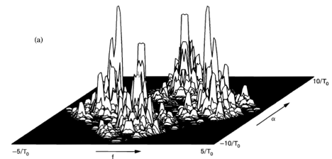
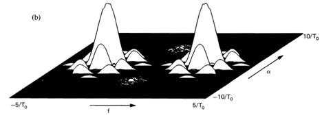
Figure 15-1 Spectral correlation magnitude for simulated QPSK signal, computed using the spectrally smoothed cyclic periodogram method. (a) time-series points, frequency points averaged. (b) time-series points, frequency points averaged.
===============
4 For some applications, the almost cyclostationary variance, ![\hat{E}\left\{ [w(t)-\hat{E}\{w(t)\}]{{}^{2}} \right\}](https://cyclostationarity.com/wp-content/ql-cache/quicklatex.com-babe48f07d55597d3126f36064767031_l3.svg "Rendered by QuickLaTeX.com") , might also be of interest, in which case the almost cyclostationary mean should be used for normalization. In (72), only the time averages of these two almost periodic quantities are used.
, might also be of interest, in which case the almost cyclostationary mean should be used for normalization. In (72), only the time averages of these two almost periodic quantities are used.
5 The definition of a Gaussian almost cyclostationary real time-series given in Section A is generalized to jointly Gaussian jointly almost cyclostationary pairs of complex time-series in [Brown 1987], where the generalization (76) of Isserlis’ formula is derived.
6 Formula (77) was first derived in [Brown 1987].
In Section A of this chapter, the concept of a fraction-of-time probabilistic model, which was introduced in Chapter 5, Part I for constant phenomena, is generalized for periodic and almost periodic phenomena. The generalization is not quite as straightforward as we might like because of the required construction of the composite fraction-of-time distribution (8) from the individual stationary and cyclostationary fraction-of-time distributions (2) and (4). Similarly, Wold’s isomorphism between a single time-series and a stationary ergodic stochastic process, which was explained in Part I, is generalized for almost cyclostationary cycloergodic stochastic processes. Again, the generalization is not as straightforward as we might like, but the added abstraction of the theory is apparently unavoidable. In any case, it is considerably less abstract than the probabilistic theory of cyclostationary and almost cyclostationary stochastic processes. In particular, all probabilistic concepts, such as statistical independence and expectation, obtained from the fraction-of-time model can be directly interpreted in terms of the concrete concept of sine wave extraction. Included in the generalized fraction-of-time theory presented here is the definition of a Gaussian almost cyclostationary time-series and a discussion of some of its most basic properties.
In Section B, the probabilistic model introduced in Section A is used to study the resolution, leakage, and reliability properties of cyclic spectrum measurements. It is explained that, in addition to the usual spectral resolution and leakage issues encountered with conventional spectrum measurements on stationary time-series, the novel issues of cycle resolution and cycle leakage are encountered with cyclic spectrum measurements on (almost) cyclostationary time-series. Cycle leakage can be particularly problematic with digital implementations that use time-hopped DFTs, especially when computational savings are obtained by the technique of subsampling because of the additional cycle aliasing problem it introduces. Also, it is seen that the variability behavior, although quite similar to that of conventional cross-spectrum measurements on stationary time-series, can differ for certain values of the two frequency parameters f and , as predicted by the correction term (82b) in the formula (82a) for the measurement variance. Singling out this term and dubbing it a correction makes explicit the difference between these formulas and their counterparts for purely stationary time-series; this difference arises because the additivity of variances in the variance of a sum of variables is lost when those variables are correlated. Aside from these few but important differences, the resolution, leakage, and reliability properties of cyclic spectrum measurements on almost cyclostationary time-series are the same as for spectrum and cross-spectrum measurements on stationary time-series. Consequently, much of the extensive discussions, descriptions, examples, and general results given in Chapters 5 and 7 of Part I apply here.
Viewers are referred to the three chapters and three books on applications, which are accessible at the links [Bk5], [BkC1], [BkC2], [BkC3], [B1], and [B2], for broad coverage of applications. There also are a number of conference papers on applications in the list of publications at the university of California faculty webpage.
It will be noticed in studying the recommended sources on practical applications that the relevance of the theory of cyclostationarity is most naturally conceptualized in terms of the Fraction-of-Time probability theory, not the more abstract theory of stochastic processes. Viewers are referred to Page 3 where this broad issue is addressed in detail. But there are two very direct explanations that can be succinctly given here.
Viewers are referred to the seminal tutorial article [JP36] in the IEEE Signal Processing Magazine for a detailed account of how the two basic phenomena, sine-wave regeneration and spectral redundancy, give rise to a beautiful wide-sense or 2nd-order theory of cyclostationarity. This theory has resulted in an explosion of discoveries of ways to exploit cyclostationarity in an immense variety of signal processing applications. For two companion seminal papers on the equally beautiful nth-order and strict-sense theories of cyclostationarity, viewers are referred to [JP55] and [JP34].
Cyclic parameter estimation problems are classified into two categories:
Essentially all empirical time-series analysis is done on digital computation devices and, because of this, the data to be analyzed must be in the form of discrete-time series. In the great majority of applications, the phenomena being studied involve dynamics that are continuous in time, but the measurements on dynamical quantities are either made at discrete points in time or are converted to discrete time by periodically sampling continuous-time data. For this reason, most time-series analysis, or signal processing, is implemented in discrete time and is therefore often treated analytically using the discrete-time theory of cyclostationarity.
If the period of cyclostationarity is known, it is most convenient to set the time-sampling increment equal to an integer divisor of the period. If the data supplied has some other time-sampling increment, it is best to re-sample the data, which is a standard operation in Digital Signal Processing software or hardware. However, if the period is unknown, re-sampling cannot be performed without some preprocessing to determine the period.
The data averaging techniques used in statistical signal processing of cyclostationary signals are of two types: synchronized averaging which averages data values separated in time by integer multiples of the period, and sinusoidally weighted averaging, which corresponds to computation of Fourier-series coefficients associated with the harmonic frequencies consisting of integer multiples of the fundamental frequency of cyclostationarity, which is the reciprocal of the period. These harmonic frequencies are called the cycle frequencies of cyclostationarity.
As a result of the above constraints imposed by implementation in terms of digital computation, unknown periods must be estimated using estimated cycle frequencies. In the case of Poly-cyclostationarity or Almost Cyclostationarity, there are more than one fundamental frequencies—more than one fundamental periods. Therefore, not all cycle frequencies are harmonically related. Nevertheless, once the cycle frequencies have been estimated, or one might say, “detected”, they can be partitioned into subsets for which all frequencies in each set are harmonically related. The number of subsets equals the number of fundamental periods.
It can be seen from this discussion that periods of cyclostationarity are typically not estimated directly; rather, they are deduced from the estimated cycle frequencies. The fact that the cycle frequencies corresponding to each fundamental period must be harmonically related can be used to improve the accuracy of the cycle-frequency estimates, which in practice will not automatically be harmonically related because of estimation errors. This can be done in two alternative ways: the first way is to create a cycle-frequency performance measure consisting of the reciprocal of the sum of squares of the errors in the cycle frequencies relative to the exact harmonic frequencies  for all detected harmonic numbers (integers) , where is a candidate value for the unknown period. This performance measure can then be maximized by minimizing the sum of squared errors with respect to the value of . The solution for can be shown to be the ratio of the sum over -squared to the sum over the product of and the -th harmonic frequency estimate. Using this optimum value of , the optimum estimate of the -th harmonic frequency is . The second way can, in principle, produce a more accurate estimate of the period. Here the real-valued objective functions, each maximized to optimize each cycle frequency estimate, can be added together and their sum can be maximized with respect to , where the nth-cycle frequency is expressed as .
It follows from this discussion that, in order to measure periodic statistics, like moments, cumulants, and cumulative probability distributions, estimation of unknown cycle frequencies is often the first order of business. Once the cycle frequencies have been estimated, the period(s) can be derived, and then periodic statistics can be measured. Of course, these can be measured in either of two ways:
Discussion of algorithms and references to research results on cycle-frequency estimation are available on pages 314 – 318 in [B2] and, for the associated task of synchronization, on pages 333 – 335 in [B2].
For single-sensor reception, there are a variety of methods for exploiting cyclostationarity for estimating signal parameters. There is always the possibility of applying the maximum-likelihood approach using a cyclostationary model for the signal instead of a stationarized model as has often been done prior to the development of the theory of cyclostationary signals and may still be appropriate in some applications today.
An alternative approach is to regenerate a spectral line by nonlinearly transforming the received data containing a cyclostationary signal in a manner that maximizes the signal-to-noise ratio of that spectral line with respect to the spectral-line frequency (cycle frequency) and some other parameter(s) with unknown values.
Yet another approach, more ad hoc, is to simply measure a cyclic statistic, like a cyclic autocorrelation or a cyclic spectrum (spectral correlation function), and then attempt to match it to the ideal version of the statistic obtained from a mathematical model of the signal by adjusting the value(s) in the model of the unknown signal parameter(s). That is, one can use a generalization of the classical Method of Moments by using cyclic moments with one or more cycle frequencies. For example, methods in this general class have been applied to time-delay and Doppler shift estimation [BkC3], [JP49], [JP42a], [JP42b]. A specific example is the SPECCOA algorithm for time-delay estimation [JP42a], which can be derived from the least-squares Method of Moments applied to the cyclic autocorrelation function.
For multi-sensor reception, there are more possibilities for devising useful algorithms for parameter estimation. Examples for which considerable progress has been made include direction-of-arrival estimation and source location estimation and are discussed further on page 2.5.7. See also Article 2 in [Bk5], where parameter estimation for purposes of synchronizing communications receivers to incoming signals is studied.
The study of causality of time series has important applications in fields of science and engineering such as climatology, meteorology, hydrology, oceanology, astronomy, etc. All these fields are growing in importance with regard to the survival of all existing species on Earth. A measure of the degree to which one time series causes another time series is the degree to which the present and past of the former can predict the future of the latter. The degree of predictability of the future of achievable with a linear transformation of the present and past of is determined by the degree to which the present and past of is correlated with the future of .
Similar facts hold for nonlinear transformations. It is easy to construct examples for which exact nonlinear prediction is possible even though no predictability is possible with any linear transformation. An example is  , which is exactly quadratically predictable, for every
  , but completely linearly unpredictable if has an even FOT probability density, because then all odd order moments of are zero and therefore the correlation between
  and is zero for all and
  .
.
Also, may be exactly predictable with a time-variant linear transformation of , but completely unpredictable with any time-invariant linear transformation. An example is  and
and  , where is a purely stationary time-series (it exhibits no cyclostationarity). It can be seen that is obviously exactly predictable with a linear periodically time-variant transformation because it equals a linear periodically time-variant transformation of the past of for every but it is completely unpredictable with any linear or nonlinear time-invariant transformation. To see that nonlinear time-invariant predictability is impossible, we simply observe that all the joint moments of and the past of the powers of are zero
![\[ \left\langle x^{n}\left(t-v \right)y\left( t \right) \right\rangle =\left\langle x^{n}\left(t-v \right)x\left( t-u \right)\cos\left( t \right) \right\rangle = 0,\quad\quad n=1,2,3,4,... \]](https://cyclostationarity.com/wp-content/ql-cache/quicklatex.com-6f50602ecaeca2a77583c6bb0c0cb25c_l3.svg "Rendered by QuickLaTeX.com")
because these moments equal cyclic moments of which are all zero since is purely stationary.
It follows that significant improvements in predictability of cyclostationary time series are achievable by considering periodically time-variant prediction instead of time-invariant prediction, whether such prediction is linear or nonlinear. This indicates that substantial periodically time-variant causality between time series can be found when there is little or no time-invariant causality. The same is true for poly-periodically time-variant causality. For example, the degree of causality found using the sum of incommensurate periodic transformations can be higher than that found using – 1, for all > 1.
The theory of noncausal linear Cyclic Wiener filtering can be modified to a theory of causal linear cyclic Wiener filtering and prediction in several ways. One way is to use a vector-valued stationary representation for a scalar-valued cyclostationary time series and apply multivariate causal time-invariant Wiener filtering/prediction theory. This theory provides the solution for the minimum-time-averaged-squared-error (Minimum-TASE) periodically time-variant causal linear filter or predictor. On the other hand, generalization in this manner to minimum-TASE poly-periodically time-variant prediction is not as straightforward. But another approach is more promising. By redefining the set of observations to be the original observations multiplied by cosine waves and sine waves (or complex sine waves with positive and negative frequencies) at some finite number of harmonics of the reciprocal of each incommensurate period of cyclostationarity, then the minimum-TASE time-invariant multivariate linear predictor can be sought. Toeplitz structure of the correlation matrices can be exploited for computational efficiency. Using finite-memory discrete-time linear predictors, and finite-length observation time-series, this is an exercise in finite-dimensional linear algebra although, for long time series and long memory, dimensionality can lead to numerical challenges. The set of linear equations can be easily set up using the orthogonal projection theorem (see tutorial Chap. 13 in [Bk3]) and solved with a standard software package subject to constraints on dimensionality.
Of course, the solutions for the minimum-TASE predictors described above cannot be implemented without knowledge of the required correlations between and as well as any nonlinear functions of to be used by nonlinear predictors. These correlations must be obtained from past observations of and . In addition, knowledge of cycle frequencies exhibited by the data is required; see Page 2.5.4.1.
For the state of the theory of linear prediction for cyclostationary time-series, as of the early 1990s, see Article 7 in [Bk5], and for a bibliography as of 2019, see Page 356 of the book [B2]. The most recent contribution to the theory of prediction for cyclostationary time-series is an elegant formula in terms of the spectral coherence matrix, for the improvement in predictability due to exploitation of cyclostationarity. This contribution is derived in the paper “On Infinite Past Predictability of Cyclostationary Signals” by Jaume Riba and Marc Vilà, published in IEEE Signal Processing Letters, Vol 29, pp. 647 – 651. Researchers seeking insight into theory and method for the following topics should benefit from the sources cited above: time series prediction and time series forecasting.